library(ggplot2)

te_pal <- list(forest = "#275139", green = "#2f8f63", sage = "#93a87f",
               clay = "#b5534e", gold = "#cda23f", line = "#dad9ca",
               ink = "#16241d", paper = "#f5f4ee")

theme_te <- function() {
  theme_minimal(base_size = 12) +
    theme(panel.grid.minor = element_blank(),
          panel.grid.major = element_line(colour = "#e7e6dc"),
          plot.background = element_rect(fill = "#f5f4ee", colour = NA),
          panel.background = element_rect(fill = "#f5f4ee", colour = NA),
          plot.title = element_text(face = "bold", colour = te_pal$ink),
          axis.title = element_text(colour = "#2c3a31"))
}Text and regular expressions in R
R
data cleaning
ecology tutorial
ggplot2
Pull site codes and sward heights out of free-text field notes with base R regular expressions, and measure what each pattern gets right and what it gets wrong.
The spreadsheet has one column nobody planned for. It is called comments or notes or obs, it is the last column on the right, and it is where the field crew wrote everything the form had no box for. Sward height. Which quadrat it was. Whether the fence was down. The site code, again, because the recorder was not sure the first column had been filled in. Two hundred and forty rows of it, in prose, and somewhere in there is the vegetation height measurement that the analysis needs.
A regular expression is the tool for that column. It is a small pattern language for describing the shape of a piece of text, and R has it built in: grepl, regexpr, regmatches, sub, gsub. The temptation is to treat the pattern as something that either works or does not, to check it on five rows, and to move on. That is the mistake this post is about. A pattern applied to free text is a measuring instrument pointed at a population of strings, and like any instrument it has an error rate that can be quantified: it returns values that are not there, and it fails to return values that are.
So the notes here are simulated, with the truth recorded alongside, and every pattern is scored against that truth. Cleaning the taxonomy in a species column is a different job, done in cleaning species names before you count; this post is about the tool rather than the task, and the worked example is extraction, not matching.
The notes column
Twelve grassland sites, six grazed and six ungrazed, twenty quadrats each. At every quadrat the recorder wrote one line of free text containing the site code, the quadrat number, a grazing condition word, and, most of the time, the sward height in centimetres. The fields are separated by semicolons and their order is whatever the recorder thought of first. Some lines carry extra observations that were worth writing down and are not part of the analysis: litter depth, moss depth, the height of a fence post, the distance to the boundary, a bare ground percentage.
Three things vary in how the sward height is written, and all three are taken from real field books. Most lines name it: sward 12 cm, sward height 12 cm, 12 cm sward. Some give the number and the unit without naming what was measured: about 8 cm. A few give a range rather than a value: sward 7-11 cm. The bare form is more common where the sward was short, which is the detail that matters later, because it means the lines a strict pattern will miss are not a random sample of the lines.
The site code varies too. The canonical form is two letters, a hyphen and a two-digit number, but the hyphen goes missing, the leading zero goes missing, and there is no rule that says a recorder in the rain writes the same way twice.
The notes are generated rather than borrowed, and the reason is the only reason there ever is: a generated notes column comes with a truth column. Every line knows what its sward height was before anybody wrote it down, which is what makes it possible to say that a pattern is right on 70.9251 per cent of the values it returns rather than that it looks about right. Nothing in the generator is adversarial. Every form of variation in it came out of a real field book, and the proportions are the ones that turn up: most lines regular, a minority written some other way, a handful of observations that were worth recording and are not what the analysis wants.
set.seed(20260819)

n_site <- 12
n_quad <- 20
prefix <- c("BR", "KL", "TS", "NV", "HD", "GM", "AR", "PL", "ZC", "WD", "MO", "FT")
site_code <- sprintf("%s-%02d", prefix, seq_len(n_site))
grazed <- rep(c(TRUE, FALSE), length.out = n_site)
site_mean <- ifelse(grazed, 8.5, 21.0) + rnorm(n_site, 0, 1.6)

n_note <- n_site * n_quad
dat <- data.frame(site = rep(site_code, each = n_quad),
                  grazed = rep(grazed, each = n_quad),
                  quadrat = rep(seq_len(n_quad), n_site),
                  stringsAsFactors = FALSE)
h <- pmax(1.5, rnorm(n_note, rep(site_mean, each = n_quad), 3.2))
dat$height <- ifelse(runif(n_note) < 0.6, round(h), round(h, 1))

p_bare <- 0.10 + 0.45 * (dat$height < 12)
dat$form <- ifelse(runif(n_note) > 0.88, "absent",
                   ifelse(runif(n_note) < 0.07, "range",
                          ifelse(runif(n_note) < p_bare, "bare", "anchored")))

num_txt <- function(v) ifelse(v == round(v), as.character(round(v)), as.character(v))
anchored_tpl <- c("sward %s cm", "sward height %s cm", "height %s cm",
                  "%s cm sward", "sward ht %s cm", "sward height: %s cm")
bare_tpl <- c("%s cm", "%s cm here", "about %s cm")
quad_tpl <- c("quadrat %d", "quad %d", "Q%d", "q %02d")
site_tpl <- c("%s-%02d", "%s-%02d", "%s-%02d", "%s-%02d", "%s-%02d",
              "%s%02d", "%s-%d")

decoy_field <- function() {
  k <- sample(1:6, 1)
  if (k == 1) paste0("litter ", num_txt(round(runif(1, 1, 6), 1)), " cm")
  else if (k == 2) paste0("dung ", num_txt(round(runif(1, 1, 4), 1)), " cm")
  else if (k == 3) paste0("moss ", num_txt(round(runif(1, 1, 5), 1)), " cm")
  else if (k == 4) paste0(sample(c(5:40, 60, 80, 120, 150, 200, 250), 1),
                          " m from fence")
  else if (k == 5) paste0("bare ground ", sample(5:95, 1), " %")
  else paste0(sample(c("fence post", "old fence", "tussock", "shrub"), 1), " ",
              sample(70:160, 1), " cm")
}

dat$note <- NA_character_
dat$site_txt <- NA_character_
for (i in seq_len(n_note)) {
  k <- match(dat$site[i], site_code)
  dat$site_txt[i] <- sprintf(sample(site_tpl, 1), prefix[k], k)
  fields <- c(paste0("site: ", dat$site_txt[i]),
              sprintf(sample(quad_tpl, 1), dat$quadrat[i]),
              if (dat$grazed[i])
                sample(c("grazed", "recently grazed", "heavily grazed"), 1)
              else sample(c("ungrazed", "not grazed", "no stock"), 1))
  if (dat$form[i] == "anchored") {
    fields <- c(fields, sprintf(sample(anchored_tpl, 1), num_txt(dat$height[i])))
  } else if (dat$form[i] == "bare") {
    fields <- c(fields, sprintf(sample(bare_tpl, 1), num_txt(dat$height[i])))
  } else if (dat$form[i] == "range") {
    w <- sample(1:3, 1)
    lo <- round(dat$height[i] - w)
    hi <- round(dat$height[i] + w)
    fields <- c(fields, paste0("sward ", num_txt(lo), "-", num_txt(hi), " cm"))
    dat$height[i] <- (lo + hi) / 2
  }
  nd <- sample(0:2, 1, prob = c(0.45, 0.4, 0.15))
  if (nd > 0) fields <- c(fields, replicate(nd, decoy_field()))
  dat$note[i] <- paste(sample(fields), collapse = "; ")
}
dat$recorded <- dat$form != "absent"
truth <- ifelse(dat$recorded, dat$height, NA_real_)

print(head(dat$note, 8))
[1] "q 01; sward height: 14 cm; site: BR-01; grazed"
[2] "about 11 cm; site: BR-01; bare ground 89 %; quadrat 2; recently grazed"
[3] "site: BR01; moss 2.1 cm; recently grazed; Q3; about 8.3 cm"
[4] "grazed; site: BR-1; q 04; sward 6-10 cm"
[5] "site: BR-01; 19 cm sward; quad 5; grazed"
[6] "site: BR-01; grazed; q 06; sward height: 8.6 cm"
[7] "about 7.9 cm; site: BR-01; quad 7; recently grazed"
[8] "site: BR01; quad 8; dung 1.6 cm; about 11 cm; litter 3.4 cm; grazed" print(table(dat$form))
  absent anchored     bare    range
28 142 59 11 round(c(notes = n_note, sites = n_site, quadrats_per_site = n_quad,
sward_height_recorded = sum(dat$recorded),
no_height_on_the_line = sum(!dat$recorded),
mean_true_height_cm = mean(truth, na.rm = TRUE),
codes_written_in_the_canonical_form = sum(dat$site_txt == dat$site),
codes_written_some_other_way = sum(dat$site_txt != dat$site)), 4) notes sites
240.0000 12.0000
quadrats_per_site sward_height_recorded
20.0000 212.0000
no_height_on_the_line mean_true_height_cm
28.0000 15.1156
codes_written_in_the_canonical_form codes_written_some_other_way
186.0000 54.0000 Of the 240 lines, 212 carry a sward height and 28 do not. Of the 212, 142 name the measurement, 59 give it in the bare form and 11 give a range, for which the honest reading is the midpoint of the two endpoints and that is what the truth column holds. The site code is written canonically on 186 lines and some other way on 54.
Two helpers do all the extraction work in this post. regexpr returns the position of the first match in each string, and with perl = TRUE it also attaches the position of every capture group, which is how you get at the part of the match you actually wanted rather than the whole of it. The second helper converts a captured string to a number only if the whole string looks like a number, so that a failed extraction becomes NA rather than a warning.
cap <- function(x, pat, g = 1) {
  m <- regexpr(pat, x, perl = TRUE)
  out <- rep(NA_character_, length(x))
  hit <- m > 0
  if (!any(hit)) return(out)
  st <- attr(m, "capture.start")[, g]
  ln <- attr(m, "capture.length")[, g]
  ok <- hit & ln > 0
  out[ok] <- substr(x[ok], st[ok], st[ok] + ln[ok] - 1)
  out
}

as_num <- function(s) {
  v <- rep(NA_real_, length(s))
  g <- !is.na(s) & grepl("^[0-9]+(\\.[0-9]+)?$", s)
  v[g] <- as.numeric(s[g])
  v
}

demo <- c("site: BR-01; sward height 14 cm; grazed",
          "q 04; litter 3.2 cm; about 6 cm; site: KL-02")
print(cap(demo, "([0-9]+(?:\\.[0-9]+)?)\\s*cm"))
[1] "14" "3.2"print(cap(demo, "site: ([^;]*)"))[1] "BR-01" "KL-02"print(as_num(cap(demo, "([0-9]+(?:\\.[0-9]+)?)\\s*cm")))[1] 14.0 3.2The pieces of pattern syntax used from here on are few. [0-9] is a character class, one character from the set; + means one or more of the thing before it; ? after a quantifier makes it lazy, matching as little as possible; . is any character; \\s is any whitespace; (...) captures; (?:...) groups without capturing; [^;] is any character that is not a semicolon. In R the backslash has to be doubled inside a string literal, so the pattern the engine sees as \s is written "\\s". That doubling is the single most common reason a pattern that worked on a website does not work in R.
In practice many people reach for the stringr package here, which wraps the same engine in a set of verbs with a consistent argument order. The pattern language underneath is identical, which is why this post spends its effort on the pattern rather than the wrapper. The stringr form is not run here because this post has to render with nothing installed beyond ggplot2:
# what the same two extractions look like with the stringr package
library(stringr)
str_match(notes, "(?:sward|height)[^0-9;]{0,10}([0-9]+(?:\\.[0-9]+)?)\\s*cm")[, 2]
str_extract(notes, "(?<=site: )[^;]+")
Three patterns and their measurement error
Here are three attempts at the sward height, in increasing order of strictness.
The first takes the first run of digits anywhere on the line. This is what a pattern looks like when someone has been told that [0-9]+ finds numbers and has not thought about which number.
The second requires the number to be followed by cm. That is a real improvement: it will not return a quadrat number or a site number. It has no opinion about which centimetre measurement it is looking at.
The third requires an anchor word. The number has to be preceded, within ten non-digit characters, by sward, height or ht, and followed by cm. A second pattern catches the reversed word order, 12 cm sward, and is applied only to the lines the first one did not match. Building a pattern in layers like this is easier to read and easier to score than one long alternation.
pat_digits   <- "([0-9]+)"
pat_cm       <- "([0-9]+(?:\\.[0-9]+)?)\\s*cm"
pat_anchored <- "(?:sward|height|ht)[^0-9;]{0,10}([0-9]+(?:\\.[0-9]+)?)\\s*cm"
pat_reversed <- "([0-9]+(?:\\.[0-9]+)?)\\s*cm\\s*sward"

x_digits <- as_num(cap(dat$note, pat_digits))
x_cm     <- as_num(cap(dat$note, pat_cm))
x_anch   <- as_num(cap(dat$note, pat_anchored))
alt      <- as_num(cap(dat$note, pat_reversed))
x_anch[is.na(x_anch)] <- alt[is.na(x_anch)]

score <- function(x) {
  got <- !is.na(x)
  right <- got & !is.na(truth) & abs(x - truth) < 1e-9
  c(returned = sum(got), correct = sum(right),
    precision = 100 * sum(right) / sum(got),
    recall = 100 * sum(right) / sum(!is.na(truth)),
    false_positives = sum(got & !right),
    misses = sum(!is.na(truth) & is.na(x)))
}
pat_names <- c("Any digits", "Any cm value", "Anchored on sward")
res <- rbind(score(x_digits), score(x_cm), score(x_anch))
rownames(res) <- pat_names
print(round(res, 4))
returned correct precision recall false_positives misses
Any digits 240 44 18.3333 20.7547 196 0
Any cm value 227 161 70.9251 75.9434 66 0
Anchored on sward 142 142 100.0000 66.9811 0 70round(c(reversed_order_lines_rescued = sum(is.na(as_num(cap(dat$note, pat_anchored)))
& !is.na(alt)),
anchored_misses_that_are_bare_form = sum(is.na(x_anch) & dat$form == "bare"),
anchored_misses_that_are_ranges = sum(is.na(x_anch) & dat$form == "range"),
cm_pattern_fires_on_a_line_with_no_height =
sum(!is.na(x_cm) & is.na(truth))), 4) reversed_order_lines_rescued
18
anchored_misses_that_are_bare_form
59
anchored_misses_that_are_ranges
11
cm_pattern_fires_on_a_line_with_no_height
15 cm_hits <- lengths(regmatches(
dat$note, gregexpr("[0-9]+(?:\\.[0-9]+)?\\s*cm", dat$note, perl = TRUE)))
round(c(lines_with_at_least_one_cm_value = sum(cm_hits > 0),
lines_with_more_than_one_cm_value = sum(cm_hits > 1),
most_cm_values_on_a_single_line = max(cm_hits),
mean_cm_values_per_line = mean(cm_hits)), 4) lines_with_at_least_one_cm_value lines_with_more_than_one_cm_value
227.000 103.000
most_cm_values_on_a_single_line mean_cm_values_per_line
3.000 1.475 Before the scores, one number explains why the choice of pattern matters at all. 227 lines carry at least one centimetre value and 103 carry more than one, up to 3 on a single line, an average of 1.4750. regexpr returns the first match and nothing else, so on 103 of the 240 lines the pattern is not finding a value, it is choosing between values, and the pattern decides which one by where it starts looking. That decision is invisible in the output and is the whole subject of this section. gregexpr returns them all, which is the right tool when you want every match, and the wrong one here because a quadrat has one sward height.
Precision is the share of the values a pattern returns that are the right value. Recall is the share of the values that were there that it returned correctly. They are not the same question and a pattern can be good at one and poor at the other. The pair comes from information retrieval and transfers to extraction without alteration, as long as you remember what the denominators are: precision divides by what the pattern returned, recall by what was there to find.
pr_df <- data.frame(
  pattern = factor(rep(pat_names, 2), levels = pat_names),
  value = c(res[, "precision"], res[, "recall"]),
  panel = factor(rep(c("Precision (per cent of returned values correct)",
                       "Recall (per cent of recorded heights found)"),
                     each = 3),
                 levels = c("Precision (per cent of returned values correct)",
                            "Recall (per cent of recorded heights found)")))

ggplot(pr_df, aes(pattern, value, fill = pattern)) +
  geom_col(width = 0.62, show.legend = FALSE) +
  geom_text(aes(label = sprintf("%.1f", value)), vjust = -0.45, size = 3.4,
            colour = te_pal$ink) +
  facet_wrap(~panel) +
  scale_fill_manual(values = c(te_pal$sage, te_pal$gold, te_pal$forest)) +
  scale_y_continuous(limits = c(0, 118), expand = c(0, 0)) +
  labs(x = NULL, y = NULL,
       title = "A pattern has an error rate, and the two errors move separately") +
  theme_te() +
  theme(strip.text = element_text(colour = te_pal$ink, face = "bold", size = 9))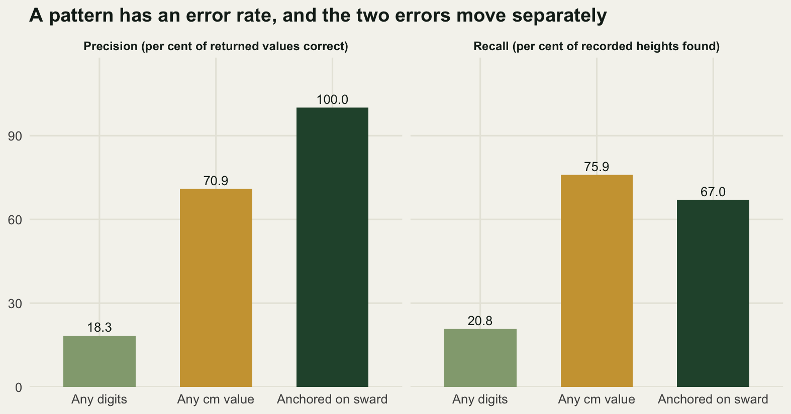
The first pattern returns a number on all 240 lines and is right on 44 of them. Precision 18.3333 per cent, recall 20.7547 per cent. It is not a bad extractor of sward height, it is not an extractor of sward height at all: what it mostly returns is the two digits of the site code, or the quadrat number, whichever the recorder happened to write first. The thing to notice is that it never complains. Every row has a number in it, the column is complete, and nothing about the output says that four fifths of it is furniture.
The second pattern returns 227 values, of which 161 are right: precision 70.9251 per cent, recall 75.9434 per cent. Both go up by a large margin for one small addition to the pattern. The 66 wrong values are litter depths, moss depths, dung pats, fence posts, tussocks and the upper end of the lines that gave a range, and 15 of them are on lines that never recorded a sward height at all, so the pattern has invented a measurement for a quadrat where none was taken.
The third returns 142 values and every one of them is correct. Precision 100 per cent. The price is recall, which falls to 66.9811 per cent: 70 recorded heights are not found, 59 of them written in the bare form and 11 written as a range. The reversed word order pattern rescues 18 lines the main one missed, which is the second layer earning its place, and it is worth seeing how small that second layer is. It is the same pattern with the two halves exchanged, applied only to the lines that came back empty. Writing it as one alternation instead would have saved nothing and would have made the whole thing harder to score, because a single pattern gives you a single number.
It is worth reading the anchored pattern once, slowly, because everything else in this post is a variation on it. (?:sward|height|ht) is the anchor: one of three words, in a group that does not capture, so the numbering of the capture groups is not disturbed by it. [^0-9;]{0,10} is the gap the recorder is allowed to leave between the anchor word and the number: up to ten characters, none of which may be a digit or a semicolon. Excluding the digit stops the pattern skipping over one number to reach another; excluding the semicolon stops it reaching across a field boundary into the next observation entirely, which is the same failure the greedy quantifier makes later on and is worth blocking twice. ([0-9]+(?:\\.[0-9]+)?) is the number, an optional decimal part included, and it is the only capturing group, which is why cap can take group one and know what it has. \\s*cm is the unit, with any amount of space or none, because 12cm and 12 cm are both in the notes.
What a wrong extraction does to the ecology
None of that matters yet. Precision and recall are properties of the extraction step, and the question that decides which pattern to ship is what they do to the number the study reports. Here that number is the difference in mean sward height between the ungrazed and the grazed sites, the whole point of the survey.
site_mean_of <- function(v) tapply(v, dat$site, function(z) mean(z, na.rm = TRUE))
gz <- tapply(dat$grazed, dat$site, function(z) z[1])
contrast <- function(m) mean(m[!gz]) - mean(m[gz])

mean_true <- site_mean_of(truth)
mean_cm   <- site_mean_of(x_cm)
mean_anch <- site_mean_of(x_anch)

round(c(overall_mean_true = mean(truth, na.rm = TRUE),
        overall_mean_cm_pattern = mean(x_cm, na.rm = TRUE),
        overall_mean_anchored = mean(x_anch, na.rm = TRUE),
        grazing_contrast_true_cm = contrast(mean_true),
        grazing_contrast_cm_pattern = contrast(mean_cm),
        grazing_contrast_anchored = contrast(mean_anch),
        attenuation_cm_pattern_percent =
          100 * (1 - contrast(mean_cm) / contrast(mean_true)),
        attenuation_anchored_percent =
          100 * (1 - contrast(mean_anch) / contrast(mean_true)),
        worst_site_error_cm_pattern = max(abs(mean_cm - mean_true)),
        worst_site_error_anchored = max(abs(mean_anch - mean_true)),
        mean_lift_at_the_grazed_sites_cm = mean(mean_cm[gz] - mean_true[gz]),
        mean_lift_at_the_ungrazed_sites_cm = mean(mean_cm[!gz] - mean_true[!gz]),
        highest_reported_site_mean_cm = max(mean_cm),
        its_true_value_cm = mean_true[which.max(mean_cm)]), 4)
overall_mean_true overall_mean_cm_pattern
15.1156 23.0515
overall_mean_anchored grazing_contrast_true_cm
17.0021 14.0461
grazing_contrast_cm_pattern grazing_contrast_anchored
4.9155 13.5462
attenuation_cm_pattern_percent attenuation_anchored_percent
65.0044 3.5584
worst_site_error_cm_pattern worst_site_error_anchored
33.4433 2.1300
mean_lift_at_the_grazed_sites_cm mean_lift_at_the_ungrazed_sites_cm
12.9004 3.7698
highest_reported_site_mean_cm its_true_value_cm.HD-05
41.4647 8.0214 site_df <- data.frame(
truth = rep(as.numeric(mean_true), 2),
reported = c(as.numeric(mean_cm), as.numeric(mean_anch)),
pattern = factor(rep(c("Any cm value", "Anchored on sward"), each = n_site),
levels = c("Any cm value", "Anchored on sward")))
ggplot(site_df, aes(truth, reported, colour = pattern, shape = pattern)) +
geom_abline(slope = 1, intercept = 0, linetype = 2, colour = te_pal$sage,
linewidth = 0.8) +
geom_point(size = 3.4, stroke = 1.1) +
scale_colour_manual(values = c(te_pal$gold, te_pal$forest), name = NULL) +
scale_shape_manual(values = c(17, 16), name = NULL) +
scale_x_continuous(limits = c(3, 43), breaks = seq(5, 40, 5)) +
scale_y_continuous(limits = c(3, 43), breaks = seq(5, 40, 5)) +
labs(x = "True mean sward height at the site (cm)",
y = "Mean reported by the pattern (cm)",
title = "The unanchored pattern lifts the short-sward sites furthest") +
theme_te() +
theme(legend.position = "top")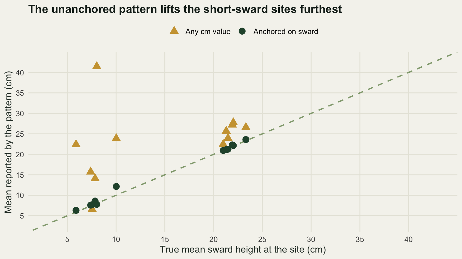
The true difference between the ungrazed and grazed site means is 14.0461 cm. The anchored pattern reports 13.5462 cm, an attenuation of 3.5584 per cent, which is the cost of losing 70 lines. On this dataset the unanchored pattern reports 4.9155 cm, an attenuation of 65.0044 per cent, so a survey designed to measure a grazing effect would report a third of it.
The mechanism is visible in the figure, and it is not the one I expected before running it. A false positive substitutes a value that has nothing to do with the site: a fence post is 80 cm high whether it stands in a grazed sward or an ungrazed one. The scatter of the wrong values is therefore about the same at every site, but its effect is not, because it is added to a small number at the grazed sites and a large one at the ungrazed sites. On this run the grazed site means are lifted by 12.9004 cm on average and the ungrazed ones by 3.7698 cm, and one grazed site whose true mean sward is 8.0214 cm is reported at 41.4647 cm. The gradient is eaten from the bottom. That is where the mechanism points, and with only a few wrong values at each site a single survey can land the other way.
The overall mean goes the same way and rises, from 15.1156 cm to 23.0515 cm, because the tussocks and fence posts are taller than the grass. An analyst who sanity-checked the overall mean and found it too high might well conclude that the sward was tall that year.
The two error types are not the same size, and the comparison is worth making carefully, because the instinct in the field is to be strict and accept the losses. Take the 66 false positives the unanchored pattern makes and repair them one at a time, leaving everything else alone, then do the same for the misses; the change in the reported mean attributable to each kind is then separable. The 70 misses of the anchored pattern get the same treatment, and to see how much of their cost comes from the missingness being non-random, the same number of lines is dropped at random from the truth, a thousand times over.
fp <- !is.na(x_cm) & (is.na(truth) | abs(x_cm - truth) > 1e-9)
miss_cm <- !is.na(truth) & is.na(x_cm)
x_fixed_fp <- x_cm
x_fixed_fp[fp] <- truth[fp]

miss_anch <- !is.na(truth) & is.na(x_anch)
truth_after_anchored_misses <- truth
truth_after_anchored_misses[miss_anch] <- NA

set.seed(4711)
random_drop <- replicate(1000, {
  v <- truth
  v[sample(which(!is.na(truth)), sum(miss_anch))] <- NA
  mean(v, na.rm = TRUE) - mean(truth, na.rm = TRUE)
})

bias_fp <- mean(x_cm, na.rm = TRUE) - mean(truth, na.rm = TRUE)
bias_fp_only <- mean(x_fixed_fp, na.rm = TRUE) - mean(truth, na.rm = TRUE)
bias_miss <- mean(truth_after_anchored_misses, na.rm = TRUE) -
  mean(truth, na.rm = TRUE)

round(c(false_positives = sum(fp),
        misses_of_the_cm_pattern = sum(miss_cm),
        misses_of_the_anchored_pattern = sum(miss_anch),
        bias_from_false_positives_cm = bias_fp,
        bias_left_when_they_are_repaired = bias_fp_only,
        bias_from_the_anchored_misses_cm = bias_miss,
        cost_per_false_positive_cm = bias_fp / sum(fp),
        cost_per_miss_cm = bias_miss / sum(miss_anch),
        ratio_of_the_two = (bias_fp / sum(fp)) / (bias_miss / sum(miss_anch)),
        random_dropout_mean_shift_cm = mean(random_drop),
        random_dropout_sd_cm = sd(random_drop),
        random_dropout_worst_of_a_thousand_cm = max(abs(random_drop)),
        rows_left_by_the_anchored_pattern = sum(!is.na(x_anch)),
        rows_left_by_the_cm_pattern = sum(!is.na(x_cm))), 4)
false_positives misses_of_the_cm_pattern
66.0000 0.0000
misses_of_the_anchored_pattern bias_from_false_positives_cm
70.0000 7.9360
bias_left_when_they_are_repaired bias_from_the_anchored_misses_cm
0.0000 1.8865
cost_per_false_positive_cm cost_per_miss_cm
0.1202 0.0270
ratio_of_the_two random_dropout_mean_shift_cm
4.4616 0.0116
random_dropout_sd_cm random_dropout_worst_of_a_thousand_cm
0.3653 1.4353
rows_left_by_the_anchored_pattern rows_left_by_the_cm_pattern
142.0000 227.0000 Repairing the 66 false positives removes the whole of the bias: 7.9360 cm before, 0 cm after, because the unanchored pattern has no misses at all. Every line that recorded a height has a cm on it somewhere, so the pattern always finds something; it just does not always find the right thing.
Each false positive moves the reported mean by 0.1202 cm. Each miss of the anchored pattern moves it by 0.0270 cm, and that number is not small because misses are inherently expensive but because these misses are concentrated on the short swards: the 70 misses together shift the mean by 1.8865 cm, while dropping the same 70 values at random from the truth shifts it by 0.0116 cm on average across a thousand draws, with a standard deviation of 0.3653 cm and a worst case of 1.4353 cm. So a false positive costs 4.4616 times what a non-random miss costs, and a miss that is random with respect to the ecology costs nothing at all beyond the loss of precision that comes with a smaller sample.
That ratio understates the asymmetry, because it prices only the bias. A miss leaves a hole. The anchored pattern returns 142 values and the row count says 142, so anybody who looks at the column sees 98 of the 240 cells empty and can decide what to do about it. The unanchored pattern returns 227 values and the row count says 227, and there is nothing anywhere in the output that distinguishes a sward height from a fence post. The strict pattern fails in a way you can see. That is the property to optimise for when you cannot have both.
Greedy, lazy, and a character class
The other classic way to lose a field is to ask for too much of the line. The site code sits between site: and the next semicolon, and there are three ways to say so.
g_greedy <- cap(dat$note, "site: (.*);")
g_lazy   <- cap(dat$note, "site: (.*?);")
g_class  <- cap(dat$note, "site: ([^;]*)")

gscore <- function(v) c(
  matched = sum(!is.na(v)),
  correct = sum(!is.na(v) & v == dat$site_txt),
  swallowed_the_next_field = sum(!is.na(v) & nchar(v) > nchar(dat$site_txt)),
  no_match = sum(is.na(v)),
  mean_characters_captured = mean(nchar(v), na.rm = TRUE))

greedy_res <- rbind(`.* greedy` = gscore(g_greedy),
                    `.*? lazy` = gscore(g_lazy),
                    `[^;]* class` = gscore(g_class))
print(round(greedy_res, 4))
matched correct swallowed_the_next_field no_match
.* greedy 190 52 138 50
.*? lazy 190 190 0 50
[^;]* class 240 240 0 0
mean_characters_captured
.* greedy 21.2895
.*? lazy 4.7579
[^;]* class 4.7750site_is_last <- !grepl("site: [^;]*;", dat$note)
extra_semicolons <- sapply(g_greedy[!is.na(g_greedy)], function(s)
lengths(regmatches(s, gregexpr(";", s, fixed = TRUE))))
round(c(site_field_written_last = sum(site_is_last),
mean_extra_fields_inside_a_greedy_capture = mean(extra_semicolons),
greedy_capture_mean_characters = mean(nchar(g_greedy), na.rm = TRUE),
true_code_mean_characters = mean(nchar(dat$site_txt))), 4) site_field_written_last
50.0000
mean_extra_fields_inside_a_greedy_capture
1.3105
greedy_capture_mean_characters
21.2895
true_code_mean_characters
4.7750 print(head(g_greedy[!is.na(g_greedy)], 3))[1] "BR-01"
[2] "BR-01; bare ground 89 %; quadrat 2"
[3] "BR01; moss 2.1 cm; recently grazed; Q3"gl <- c("Correct", "Swallowed the next field", "No match")
# the outcome palette, kept apart from the pattern palette used in the earlier
# figures: green right, clay wrong, ink for the lines that came back empty. The
# in-bar count takes whichever text colour reads on the fill under it.
pal_outcome <- c(te_pal$green, te_pal$clay, te_pal$ink)
lab_outcome <- c(te_pal$ink, te_pal$paper, te_pal$paper)
greedy_df <- data.frame(
pattern = factor(rep(rownames(greedy_res), each = 3),
levels = rev(rownames(greedy_res))),
outcome = factor(rep(gl, 3), levels = gl),
n = as.numeric(t(cbind(greedy_res[, "correct"],
greedy_res[, "swallowed_the_next_field"],
greedy_res[, "no_match"]))))
ggplot(greedy_df, aes(n, pattern, fill = outcome)) +
geom_col(width = 0.6, position = position_stack(reverse = TRUE)) +
geom_text(aes(label = ifelse(n > 0, n, ""), colour = outcome),
position = position_stack(vjust = 0.5, reverse = TRUE), size = 3.4,
fontface = "bold", show.legend = FALSE) +
scale_fill_manual(values = pal_outcome, name = NULL) +
scale_colour_manual(values = lab_outcome, guide = "none") +
scale_x_continuous(expand = expansion(mult = c(0, 0.02))) +
labs(x = "Field note lines", y = NULL,
title = "The greedy quantifier runs past the field on 138 of 240 lines") +
theme_te() +
theme(legend.position = "top")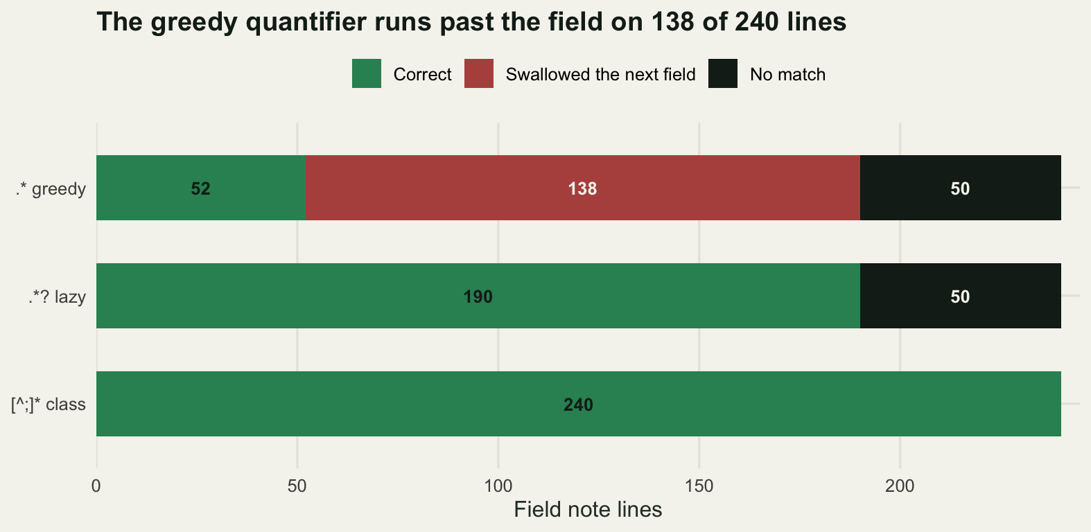
.* is greedy: it takes as much of the line as it can and then gives characters back only until the rest of the pattern can match. The rest of the pattern here is a semicolon, so it gives back only as far as the last semicolon on the line, not the first. On the 190 lines where a semicolon follows the site field it therefore captures the code and every field between it and the end, an average of 21.2895 characters where the code is 4.7750, with 1.3105 extra field separators inside the capture. It is correct on 52 of those lines, the ones where the site field happened to be the second to last.
.*? is lazy: same pattern, one character added, and it takes as little as it can. It captures the site code and stops at the first semicolon, correct on all 190 lines it matches.
Both fail on the same 50 lines, the ones where the recorder wrote the site code last and there is no semicolon after it. A greedy or lazy .* followed by ; needs that semicolon to exist. [^;]* does not: it says “characters that are not a semicolon”, and it stops at a semicolon or at the end of the line, whichever comes first. It matches all 240 lines and is correct on all 240.
The lesson generalises past this example. When you know what the field cannot contain, say that, rather than saying “anything” and then adding a boundary. A character class carries the field definition inside it; .* plus a delimiter is two claims that have to agree, and on the last field of a line they do not.
The same argument decides between the other base R text functions. grepl answers whether the pattern is there and returns a logical, which is what you want for a flag and never enough for a value. sub replaces the first match and gsub replaces every match, so gsub on a pattern that matches more than you meant edits more of the line than you meant, quietly and everywhere at once. regexpr with capture groups, which is what cap wraps, is the one that hands back the piece of the line you asked for and leaves the rest alone. When an extraction goes wrong it is usually because a replacement was used where a capture was wanted: the difference is that a capture cannot damage the source text, and a replacement can, and the damaged version is the one that gets saved.
Nothing is extracted until it is checked
Two more fields are buried in the same lines, and both are easier than the sward height in the sense that matters least. They look like they cannot go wrong.
The grazing condition is a word, not a number, so grepl is enough and there is nothing to parse. The trap is that one of the words the recorder used contains another: ungrazed contains grazed, and so does not grazed, in a different way. The quadrat number sits behind one of four spellings, quadrat 7, quad 7, Q7 and q 07, and comes out as a string in which the last of those four does not equal the other three.
flag_naive <- grepl("grazed", dat$note)
flag_word  <- grepl("\\bgrazed\\b", dat$note)
flag_care  <- grepl("\\bgrazed\\b", dat$note) &
  !grepl("ungrazed|not grazed|no stock", dat$note)

flag_score <- function(f) c(
  called_grazed = sum(f),
  correct = sum(f == dat$grazed),
  ungrazed_lines_called_grazed = sum(f & !dat$grazed),
  accuracy_percent = 100 * mean(f == dat$grazed))
flag_names <- c("grepl grazed", "word boundary", "with the exclusions")
flags <- rbind(flag_score(flag_naive), flag_score(flag_word), flag_score(flag_care))
rownames(flags) <- flag_names
print(round(flags, 4))
called_grazed correct ungrazed_lines_called_grazed
grepl grazed 202 158 82
word boundary 155 205 35
with the exclusions 120 240 0
accuracy_percent
grepl grazed 65.8333
word boundary 85.4167
with the exclusions 100.0000contrast_from <- function(f)
mean(truth[!f], na.rm = TRUE) - mean(truth[f], na.rm = TRUE)
q_raw <- cap(dat$note, "(?:quadrat|quad|[Qq])\\s*([0-9]+)")
round(c(lines_grepl_grazed_does_not_claim = sum(!flag_naive),
true_contrast_from_the_recorded_flag = contrast_from(dat$grazed),
contrast_from_grepl_grazed = contrast_from(flag_naive),
contrast_from_the_word_boundary = contrast_from(flag_word),
contrast_from_the_exclusions = contrast_from(flag_care),
attenuation_grepl_grazed_percent =
100 * (1 - contrast_from(flag_naive) / contrast_from(dat$grazed)),
attenuation_word_boundary_percent =
100 * (1 - contrast_from(flag_word) / contrast_from(dat$grazed)),
quadrat_numbers_correct = sum(as_num(q_raw) == dat$quadrat),
distinct_quadrat_strings = length(unique(q_raw)),
distinct_quadrat_numbers = length(unique(as_num(q_raw))),
quadrat_strings_with_a_leading_zero = sum(grepl("^0", q_raw))), 4) lines_grepl_grazed_does_not_claim true_contrast_from_the_recorded_flag
38.0000 14.1479
contrast_from_grepl_grazed contrast_from_the_word_boundary
7.5833 10.1666
contrast_from_the_exclusions attenuation_grepl_grazed_percent
14.1479 46.4002
attenuation_word_boundary_percent quadrat_numbers_correct
28.1404 240.0000
distinct_quadrat_strings distinct_quadrat_numbers
28.0000 20.0000
quadrat_strings_with_a_leading_zero
25.0000 grepl("grazed", ...) calls 202 of the 240 lines grazed when 120 of them are. Every line that says ungrazed contains the string, and so does every line that says not grazed. The 38 lines it does not claim are the ones where the recorder wrote no stock, which is the only ungrazed wording that does not contain the word. Accuracy 65.8333 per cent, and 82 ungrazed lines end up in the grazed group. The grazing difference computed from that column is 7.5833 cm against a true line-level difference of 14.1479, an attenuation of 46.4002 per cent.
The word boundary version is better and is the dangerous one, because it looks like the fix. \\bgrazed\\b requires a word boundary on each side, so it correctly refuses ungrazed: the letters n and g are both word characters and there is no boundary between them. It cannot refuse not grazed, because there the boundary is exactly where the pattern wants it. It is right on 205 of 240 lines, an accuracy of 85.4167 per cent, and every one of the 35 lines it gets wrong is an ungrazed line moved into the grazed group. Those lines carry the tall swards. The reported difference is 10.1666 cm, an attenuation of 28.1404 per cent, from a pattern that is right five times out of six and looks careful.
The version that works states the exclusions rather than trusting the boundary, and is right on all 240 lines. That is the general shape of the fix: when one category label contains another as a substring, no amount of boundary syntax will separate them, and the pattern has to name the thing you do not want. It is also the one case in this post where the check is easier than the pattern, because a table of the extracted flag against the site would have shown, immediately, sites carrying both labels in a design where each site has exactly one.
The quadrat number comes out correct on all 240 lines once it is converted, and as a string it comes out as 28 distinct values where there are 20 quadrats, because 25 lines wrote the number with a leading zero. A join on that string matches 20 of the levels and silently drops the rest. The fix is one call to as_num, and the reason to mention something so small is that a pattern’s output is text until you convert it, and text compares as text.
The sward height needs more than a conversion, and the last question is what a cheap check catches. A range check is the cheapest thing there is: sward height in this system is between half a centimetre and 60 centimetres, so anything outside that is not a sward height. A cross-tabulation is the other cheap thing: the site codes that come out of the notes should be twelve values, the ones on the site list, and any other value is an error whether or not it looks plausible.
in_range <- function(v) !is.na(v) & v >= 0.5 & v <= 60
bad_digits <- !is.na(x_digits) & (is.na(truth) | abs(x_digits - truth) > 1e-9)

x_checked <- ifelse(in_range(x_cm), x_cm, NA_real_)
mean_checked <- site_mean_of(x_checked)

round(c(cm_pattern_wrong_values = sum(fp),
        caught_by_the_range_check = sum(fp & !in_range(x_cm)),
        surviving_the_range_check = sum(fp & in_range(x_cm)),
        digits_pattern_wrong_values = sum(bad_digits),
        digits_caught_by_the_range_check = sum(bad_digits & !in_range(x_digits)),
        digits_surviving = sum(bad_digits & in_range(x_digits)),
        smallest_surviving_value_cm = min(x_cm[fp & in_range(x_cm)]),
        median_surviving_value_cm = median(x_cm[fp & in_range(x_cm)]),
        largest_surviving_value_cm = max(x_cm[fp & in_range(x_cm)]),
        mean_before_the_check_cm = mean(x_cm, na.rm = TRUE),
        mean_after_the_check_cm = mean(x_checked, na.rm = TRUE),
        true_mean_cm = mean(truth, na.rm = TRUE),
        bias_before_cm = mean(x_cm, na.rm = TRUE) - mean(truth, na.rm = TRUE),
        bias_after_cm = mean(x_checked, na.rm = TRUE) - mean(truth, na.rm = TRUE),
        mean_absolute_error_before_cm = mean(abs(x_cm - truth), na.rm = TRUE),
        mean_absolute_error_after_cm = mean(abs(x_checked - truth), na.rm = TRUE),
        contrast_after_the_check_cm = contrast(mean_checked),
        attenuation_after_the_check_percent =
          100 * (1 - contrast(mean_checked) / contrast(mean_true))), 4)
cm_pattern_wrong_values caught_by_the_range_check
66.0000 23.0000
surviving_the_range_check digits_pattern_wrong_values
43.0000 196.0000
digits_caught_by_the_range_check digits_surviving
11.0000 185.0000
smallest_surviving_value_cm median_surviving_value_cm
1.1000 2.5000
largest_surviving_value_cm mean_before_the_check_cm
28.0000 23.0515
mean_after_the_check_cm true_mean_cm
12.7338 15.1156
bias_before_cm bias_after_cm
7.9360 -2.3817
mean_absolute_error_before_cm mean_absolute_error_after_cm
7.9769 2.3045
contrast_after_the_check_cm attenuation_after_the_check_percent
10.9214 22.2458 class_of <- function(x, bad) {
cl <- rep(NA_character_, length(x))
cl[!is.na(x) & !bad] <- "Correct"
cl[bad & in_range(x)] <- "Wrong, inside the range"
cl[bad & !in_range(x)] <- "Wrong, outside the range"
cl
}
cl_lev <- c("Correct", "Wrong, inside the range", "Wrong, outside the range")
rng_df <- rbind(
data.frame(value = x_cm, cls = class_of(x_cm, fp),
panel = "Any cm value"),
data.frame(value = x_digits, cls = class_of(x_digits, bad_digits),
panel = "Any digits"))
rng_df <- rng_df[!is.na(rng_df$value), ]
rng_df$cls <- factor(rng_df$cls, levels = cl_lev)
rng_df$panel <- factor(rng_df$panel, levels = c("Any cm value", "Any digits"))
ggplot(rng_df, aes(value, cls, colour = cls)) +
geom_vline(xintercept = c(0.5, 60), linetype = 2, colour = te_pal$ink,
linewidth = 0.6) +
annotate("text", x = 64, y = "Wrong, inside the range", hjust = 0,
vjust = -0.9, size = 3.2, colour = te_pal$ink,
label = "Range check limits: 0.5 cm and 60 cm") +
geom_point(size = 2.1, alpha = 0.8, show.legend = FALSE,
position = position_jitter(height = 0.22, width = 0, seed = 11)) +
facet_wrap(~panel, ncol = 1) +
scale_colour_manual(values = pal_outcome) +
scale_x_continuous(limits = c(0, max(rng_df$value) + 6),
breaks = seq(0, 250, 25)) +
labs(x = "Extracted value (cm)", y = NULL,
title = "A range check catches only the errors that are far away") +
theme_te() +
theme(strip.text = element_text(colour = te_pal$ink, face = "bold", size = 9))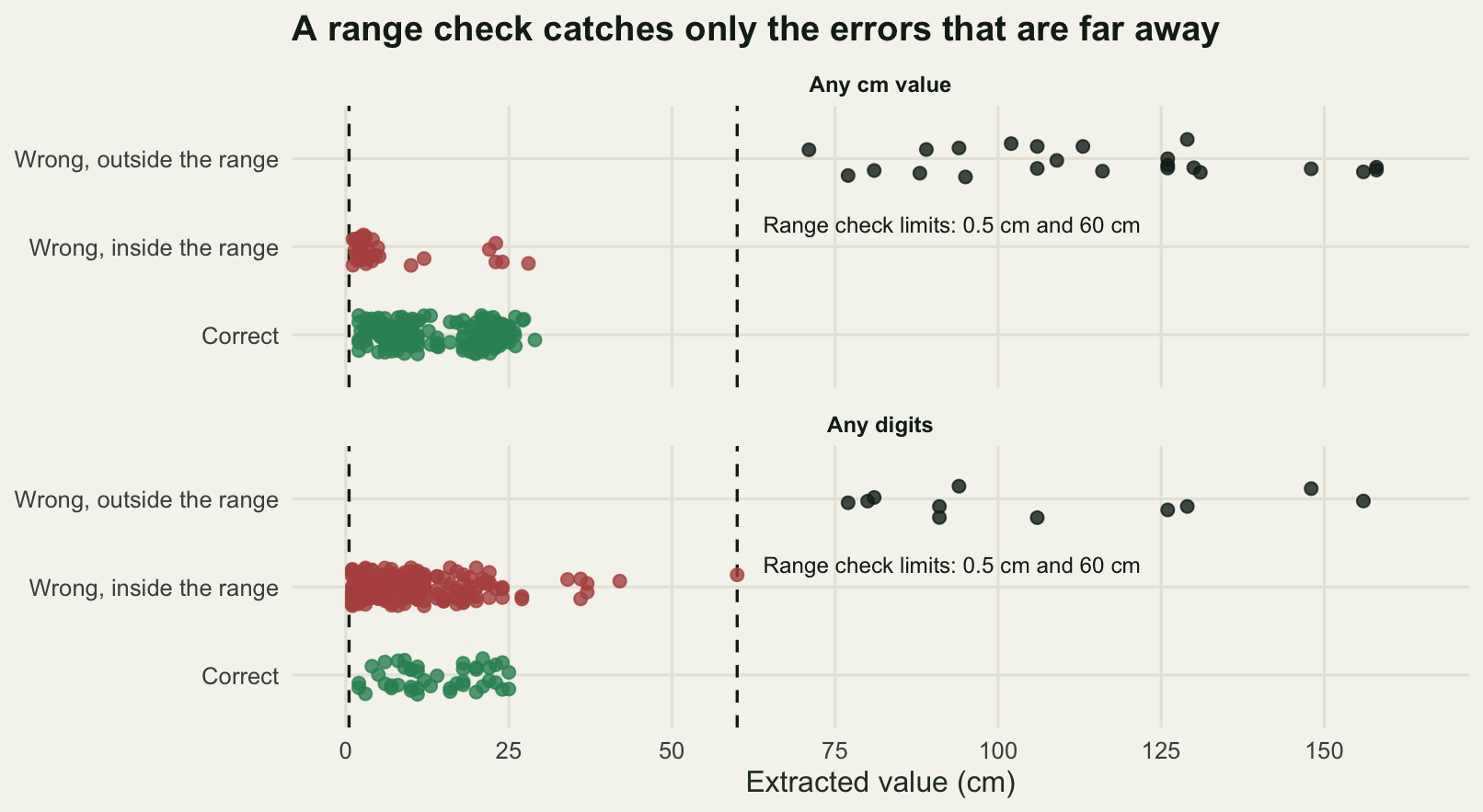
The range check catches 23 of the 66 wrong values from the unanchored pattern and lets 43 through. The ones it catches are the fence posts, the tussocks and the shrubs, all above 60 cm. The ones it lets through run from 1.1 cm to 28 cm with a median of 2.5 cm: litter depths, moss depths, dung pats and the upper ends of the lines that gave a range, every one of them a plausible sward height. A heavily grazed quadrat really can have a sward of 2 cm. No range check can separate those, because they are not outside any range.
What the check does achieve is worth having anyway. The reported mean falls from 23.0515 cm to 12.7338 cm against a truth of 15.1156, so the bias flips sign from 7.9360 cm to -2.3817 cm and its size falls; the mean absolute error per line falls from 7.9769 cm to 2.3045 cm. On this run the grazing contrast comes back from 4.9155 cm to 10.9214 cm, so the attenuation falls from 65.0044 per cent to 22.2458 per cent. Here a check that catches a third of the errors recovers most of the distortion, because the errors that are large are both the easiest to catch and the ones that do the damage. What it cannot do is finish the job. 22.2458 per cent is still a badly wrong answer, arrived at by a script in which nothing failed.
The site code check works differently and is the more useful of the two in practice, because it is not a range but a list.
code_loose  <- cap(dat$note, "site: ([A-Za-z0-9-]+)")
code_strict <- cap(dat$note, "site: ([A-Z]{2}-[0-9]{2})")

normalise <- function(s) {
  s <- toupper(s)
  s <- sub("^([A-Z]{2})-?([0-9]+)$", "\\1-\\2", s)
  sub("^([A-Z]{2})-([0-9])$", "\\1-0\\2", s)
}
code_norm <- normalise(code_loose)

kept <- !is.na(code_strict)
mean_kept <- tapply(truth[kept], dat$site[kept], function(z) mean(z, na.rm = TRUE))
gz_kept <- tapply(dat$grazed[kept], dat$site[kept], function(z) z[1])

print(sort(table(code_loose), decreasing = TRUE)[1:6])
code_loose
GM-06 PL-08 AR-07 BR-01 FT-12 KL-02
17 17 16 16 16 16 round(c(distinct_codes_the_loose_pattern_returns = length(unique(code_loose)),
codes_that_exist = n_site,
lines_whose_raw_code_is_not_on_the_site_list =
sum(!code_loose %in% site_code),
lines_the_strict_code_pattern_returns = sum(kept),
lines_the_strict_code_pattern_drops = sum(!kept),
percent_of_lines_kept = 100 * mean(kept),
exact_matches_after_normalising = sum(code_norm == dat$site),
unknown_codes_after_normalising = sum(!code_norm %in% site_code),
contrast_on_the_kept_lines_cm =
mean(mean_kept[!gz_kept]) - mean(mean_kept[gz_kept]),
contrast_on_all_lines_cm = contrast(mean_true)), 4) distinct_codes_the_loose_pattern_returns
32.0000
codes_that_exist
12.0000
lines_whose_raw_code_is_not_on_the_site_list
54.0000
lines_the_strict_code_pattern_returns
186.0000
lines_the_strict_code_pattern_drops
54.0000
percent_of_lines_kept
77.5000
exact_matches_after_normalising
240.0000
unknown_codes_after_normalising
0.0000
contrast_on_the_kept_lines_cm
13.9729
contrast_on_all_lines_cm
14.0461 The loose pattern returns 32 distinct site codes from a survey with 12 sites. That single line of table() output is the whole check, and it needs no knowledge of what went wrong: a count of levels that does not match the count of sites is a fault, full stop. 54 lines carry a code that is not on the list, and three lines of normalising, upper case, put the hyphen back, pad the number, take all 240 lines to an exact match with 0 unknown codes left.
The strict pattern is the alternative and it is worse in a specific and familiar way. It returns nothing on those 54 lines, 77.5 per cent of the survey survives, and if that extraction feeds a join onto the site table then 54 quadrats leave the analysis without any step in the script announcing that they have gone. Here the loss happens to be harmless: the contrast on the kept lines is 13.9729 cm against 14.0461 cm on all of them, because how a recorder writes a site code has nothing to do with how tall the grass is. That is luck, not design. If the sloppy writing came from the crew who worked the wet sites, the loss would carry the ecology with it, and nothing in the output would say so.
The honest limit
The measurement here scores patterns against a truth column, and the truth column exists because the notes were generated. On a real notes column there is no truth column, which is the entire difficulty. What you can do instead is read a random sample, by hand, and score the pattern against your own reading: fifty lines is enough to put a useful bound on precision, and the lines the pattern did not match are the ones to read first, because they are where the forms you did not anticipate are hiding.
The second limit is that the classes of error measured here are the ones built into the generator. Field notes contain worse. Transposed digits, a height written in inches by the one crew member who grew up with them, a comment that says the sward was measured after mowing, a line in a second language, a value the recorder later crossed out and rewrote. A pattern scored at 100 per cent precision on the errors you thought of is not scored on the errors you did not.
The third is that everything in this post extracts, and nothing here validates the ecology. The range check knows that 88 cm is not a sward height. It does not know that a 30 cm sward at a heavily grazed site is unlikely, that a quadrat was recorded twice, or that the same site appears with two different grazing words on different lines. Those need a cross-tabulation against the design rather than a check on one column, which is a different piece of work and is the one that catches the errors that survived here.
A fourth is about the engine rather than the ecology. The cap helper and the gregexpr call that counts centimetre values run with perl = TRUE, which selects the PCRE engine. The grepl and sub calls elsewhere in the post do not, so they run on the default engine instead. R ships with those two, and they agree on the constructs used here but not on everything. Lookarounds, the (?<=site: ) form that appeared in the stringr block above, are a PCRE feature and are not available in the default engine. Character class shorthands and case folding can differ. A pattern is not portable between the two by assumption, so pick one, say which, and keep the argument on every call rather than on some of them. This post did not.
And a smaller one worth saying plainly: none of this is a reason to write the pattern as a single unreadable line. The anchored extraction in this post is two patterns applied in sequence, each of which fits on one line and can be scored on its own. A pattern you cannot explain to the person who collected the data is a pattern you cannot check.
Where to go next
The obvious neighbour is cleaning species names before you count, which takes the same free-text problem in its other form: not pulling a field out of a comment, but deciding whether two spellings are the same taxon. Read that one for the matching half of the problem and this one for the extraction half. Before either, reading field data into R settles what the columns mean in the first place, including the difference between an empty cell and a recorded zero, which is the same distinction that separates a miss from a false positive here.
Once the fields are out of the notes, the dates among them are their own hazard, and dates and times in ecological data measures what a mismatched format costs when it fails silently. If you find yourself writing the same extraction in three scripts, the checks in this post are exactly the kind of statement that belongs in a test file: testing your analysis code scores what different kinds of test are worth, and a pattern with a known precision on a known set of lines is the easiest golden test you will ever write.
References
Wickham H 2014 Journal of Statistical Software 59(10):1-23 (10.18637/jss.v059.i10)
Broman KW, Woo KH 2018 The American Statistician 72(1):2-10 (10.1080/00031305.2017.1375989)
Michener WK, Jones MB 2012 Trends in Ecology and Evolution 27(2):85-93 (10.1016/j.tree.2011.11.016)
Wilson G, Bryan J, Cranston K, Kitzes J, Nederbragt L, Teal TK 2017 PLoS Computational Biology 13(6):e1005510 (10.1371/journal.pcbi.1005510)
Zizka A, Silvestro D, Andermann T, Azevedo J, Duarte Ritter C, Edler D, Farooq H, Herdean A, Ariza M, Scharn R, Svantesson S, Wengstrom N, Zizka V, Antonelli A 2019 Methods in Ecology and Evolution 10(5):744-751 (10.1111/2041-210X.13152)
Friedl JEF 2006 Mastering Regular Expressions, Third Edition, O’Reilly Media (ISBN 978-0-596-52812-6)