---
title: "What a CSV loses: archiving an R analysis"
description: "A deposited CSV round-trips the numbers and drops the structure. The fit is identical to machine precision and the reported trend changes sign. Worked in R."
date: "2026-08-06 11:00"
categories: [R, reproducibility, data management, ecology tutorial]
image: thumbnail.png
image-alt: "Two identical sets of fitted cell means, one labelled with a positive linear trend contrast and the other with a negative one of similar size."
---
The file you deposit with the paper is not the object you analysed. It is a projection of that object onto a grid of characters, and the projection is lossy in a way that R will not warn you about, because everything that survives the round trip survives it perfectly.
The numbers come back exact. The fitted model comes back exact. What does not come back is the structure you put on top of the numbers, and in the case below that structure is the whole result.
## An ordered factor, written out and read back
Cover class low, medium, high, and a Poisson count that rises across them. The analyst declared the ordering, because low, medium and high are not three arbitrary labels, and R gave them polynomial contrasts: a linear term and a quadratic term, which is exactly what an ordered predictor is for.
```{r setup}
#| message: false
#| warning: false
library(ggplot2)

te_paper  <- "#f5f4ee"
te_ink    <- "#16241d"
te_body   <- "#2c3a31"
te_forest <- "#275139"
te_rust   <- "#b5534e"
te_gold   <- "#c9b458"
te_line   <- "#dad9ca"

theme_datasheet <- function() {
  theme_minimal(base_size = 12) +
    theme(plot.background  = element_rect(fill = te_paper, colour = NA),
          panel.background = element_rect(fill = te_paper, colour = NA),
          panel.grid.major = element_line(colour = te_line, linewidth = 0.3),
          panel.grid.minor = element_blank(),
          text             = element_text(colour = te_body),
          plot.title       = element_text(colour = te_ink, face = "bold"),
          axis.text        = element_text(colour = te_body))
}

make_plots <- function(n_per = 40) {
  lev <- c("low", "medium", "high")
  d <- data.frame(cover = factor(rep(lev, each = n_per), levels = lev,
                                 ordered = TRUE))
  d$count <- rpois(nrow(d), exp(1.2 + 0.5 * (as.integer(d$cover) - 1)))
  d
}

set.seed(20260806)
field <- make_plots()
str(field$cover)
```
The analysis is one line, and the coefficient the paper would quote is the linear term.
```{r fit-before}
fit_before <- glm(count ~ cover, family = poisson, data = field)
round(coef(summary(fit_before)), 4)
```
Now archive it the way almost everyone archives it, and read it back the way the next person will.
```{r roundtrip}
path <- tempfile(fileext = ".csv")
write.csv(field, path, row.names = FALSE)

back <- read.csv(path)
back$cover <- factor(back$cover, ordered = TRUE)   # the reasonable next step
levels(back$cover)
```
There is the loss, and it is one line long. The CSV stored the labels and nothing else, so `factor` did what it always does with an unknown level set: it sorted alphabetically. High now comes first and medium last, and the ordering the ecologist declared has been replaced by the ordering of the Latin alphabet.
## The fit is identical and the answer is not
```{r fit-after}
fit_after <- glm(count ~ cover, family = poisson, data = back)

c(same_fitted  = isTRUE(all.equal(unname(fitted(fit_before)),
                                  unname(fitted(fit_after)))),
  same_loglik  = isTRUE(all.equal(as.numeric(logLik(fit_before)),
                                  as.numeric(logLik(fit_after)))))
round(c(deviance_before = deviance(fit_before),
        deviance_after  = deviance(fit_after)), 4)
```
Every diagnostic an ecologist would run passes. The fitted values agree, the deviance agrees to `r sprintf("%.4f", deviance(fit_before))` on both sides, the residual plots are the same plots. Nothing is broken, because nothing is broken: both models describe the same three group means.
```{r contrasts}
lin_before  <- coef(fit_before)[["cover.L"]]
lin_after   <- coef(fit_after)[["cover.L"]]
quad_before <- coef(fit_before)[["cover.Q"]]
quad_after  <- coef(fit_after)[["cover.Q"]]

round(c(linear_before = lin_before, linear_after = lin_after,
        quad_before = quad_before, quad_after = quad_after), 4)
```
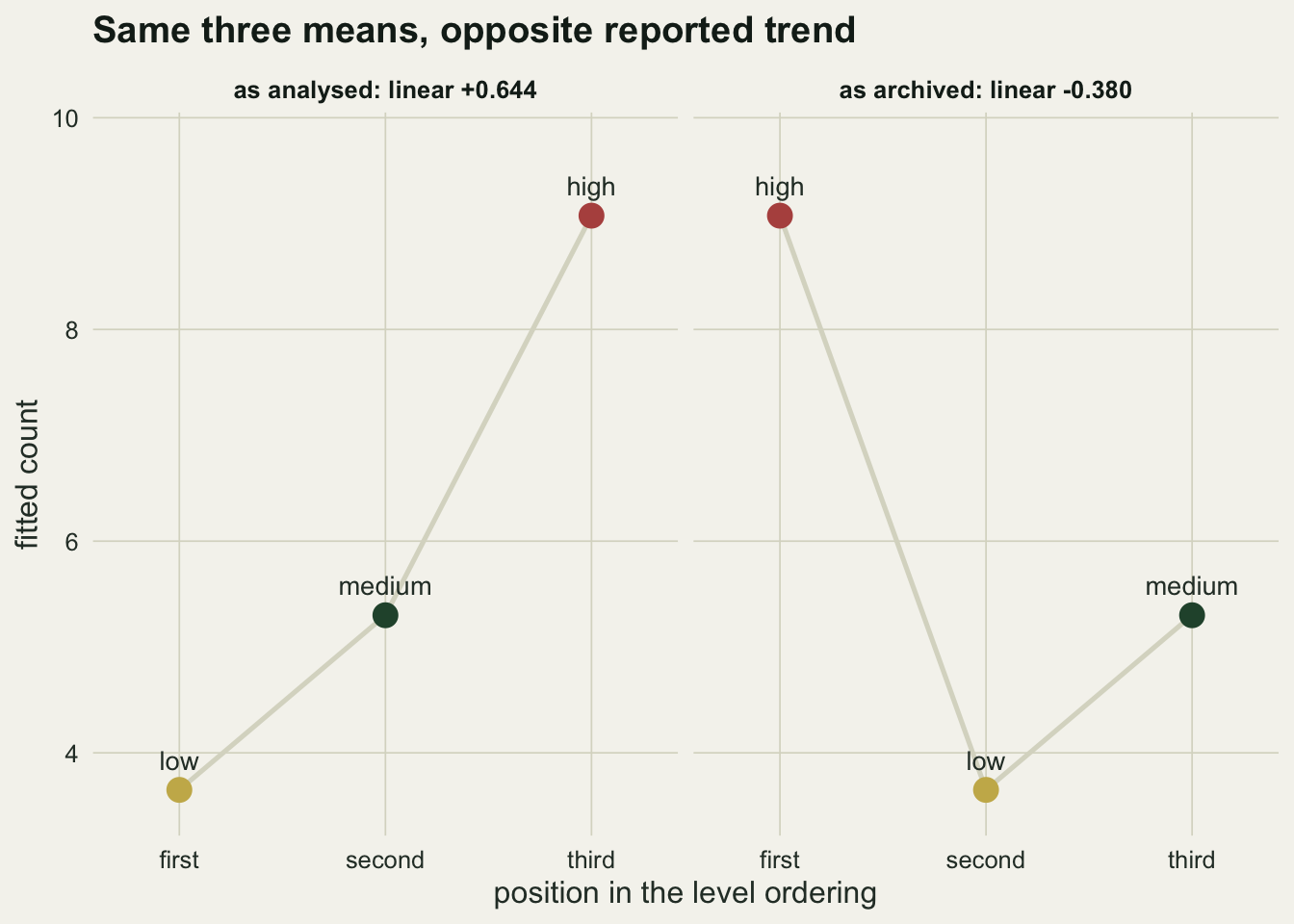
The linear contrast goes from `r sprintf("%+.4f", lin_before)` to `r sprintf("%+.4f", lin_after)`. That is the number the abstract quotes, and it has changed sign. The quadratic term moves from `r sprintf("%+.4f", quad_before)` to `r sprintf("%+.4f", quad_after)` and absorbs most of the pattern instead.
Nothing is wrong with either fit. The second one is a perfectly correct linear contrast across high, low, medium in that order, which is a sequence with no meaning at all. The archive did not corrupt the data; it dropped the sentence that said which order the levels were in.
```{r fig-means}
#| fig-cap: "Fitted counts per cover class before and after the archive round trip, with the linear polynomial contrast each fit reports."
#| fig-alt: "Two panels of three points each. The heights of the points are identical between panels, but the horizontal ordering differs, and each panel carries an annotation giving its linear contrast: positive in the left panel, negative in the right one."
pred_panel <- function(m, d, lab) {
  nd <- data.frame(cover = factor(levels(d$cover), levels = levels(d$cover),
                                  ordered = TRUE))
  nd$fit   <- predict(m, nd, type = "response")
  nd$panel <- lab
  nd$pos   <- seq_len(nrow(nd))
  nd$label <- as.character(nd$cover)
  nd
}
pan <- rbind(
  pred_panel(fit_before, field,
             sprintf("as analysed: linear %+.3f", lin_before)),
  pred_panel(fit_after, back,
             sprintf("as archived: linear %+.3f", lin_after)))
pan$panel <- factor(pan$panel, levels = unique(pan$panel))

ggplot(pan, aes(x = pos, y = fit)) +
  geom_line(linewidth = 0.9, colour = te_line) +
  geom_point(aes(colour = label), size = 4) +
  geom_text(aes(label = label), vjust = -1.1, size = 3.6, colour = te_body) +
  facet_wrap(~ panel) +
  scale_colour_manual(values = c(low = te_gold, medium = te_forest,
                                 high = te_rust)) +
  scale_x_continuous(breaks = 1:3, labels = c("first", "second", "third"),
                     expand = expansion(add = 0.42)) +
  scale_y_continuous(expand = expansion(mult = c(0.08, 0.18))) +
  labs(x = "position in the level ordering", y = "fitted count",
       title = "Same three means, opposite reported trend") +
  theme_datasheet() +
  theme(legend.position = "none",
        strip.text = element_text(colour = te_ink, face = "bold"))
```
## It is not the seed
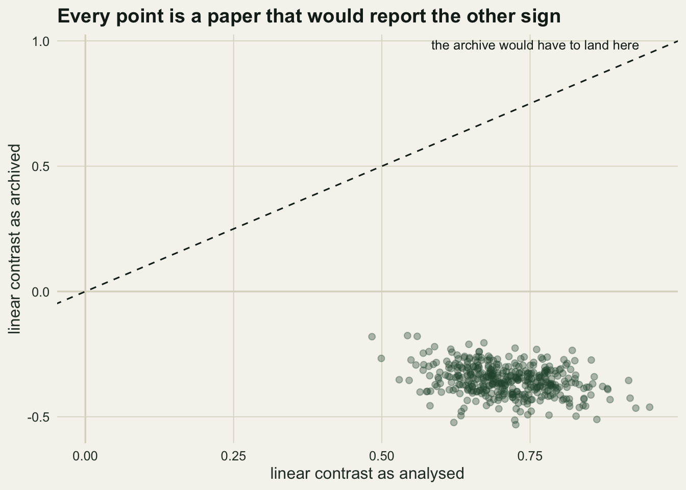
One data set proves nothing about a mechanism, so run it a few hundred times and look at the two contrasts side by side.
```{r sweep}
set.seed(7)
sw <- t(replicate(400, {
  d <- make_plots()
  b <- glm(count ~ cover, family = poisson, data = d)
  p <- tempfile(fileext = ".csv")
  write.csv(d, p, row.names = FALSE)
  r <- read.csv(p)
  r$cover <- factor(r$cover, ordered = TRUE)
  unlink(p)
  a <- glm(count ~ cover, family = poisson, data = r)
  c(before = coef(b)[["cover.L"]], after = coef(a)[["cover.L"]])
}))

round(c(mean_before   = mean(sw[, "before"]),
        mean_after    = mean(sw[, "after"]),
        sign_flips    = mean(sign(sw[, "before"]) != sign(sw[, "after"])),
        max_abs_gap   = max(abs(sw[, "before"] - sw[, "after"]))), 4)
```
Across `r nrow(sw)` archived data sets the linear contrast averages `r sprintf("%+.3f", mean(sw[, "before"]))` as analysed and `r sprintf("%+.3f", mean(sw[, "after"]))` as archived, and the sign flips in `r sprintf("%.0f", 100 * mean(sign(sw[, "before"]) != sign(sw[, "after"])))` per cent of them. The largest single discrepancy is `r sprintf("%.3f", max(abs(sw[, "before"] - sw[, "after"])))`. This is not a rare collision between a seed and an alphabet; it is what happens every time the field ordering and the alphabetical ordering disagree, which for low, medium and high they always do.
```{r fig-sweep}
#| fig-cap: "Linear contrast as analysed against the same contrast recovered from the archived file, over 400 simulated data sets."
#| fig-alt: "A scatter of four hundred points against a dashed diagonal line marking equality and a solid line at zero. No point is near the diagonal, and the cloud sits entirely in the quadrant where the analysed contrast is positive and the archived one is negative."
sw_df <- as.data.frame(sw)

ggplot(sw_df, aes(x = before, y = after)) +
  geom_hline(yintercept = 0, colour = te_line, linewidth = 0.6) +
  geom_vline(xintercept = 0, colour = te_line, linewidth = 0.6) +
  geom_abline(slope = 1, intercept = 0, linetype = "dashed", colour = te_ink) +
  geom_point(alpha = 0.35, size = 1.9, colour = te_forest) +
  annotate("text", x = max(sw_df$before), y = max(sw_df$before), hjust = 1.05,
           vjust = -0.4, size = 3.4, colour = te_ink,
           label = "the archive would have to land here") +
  labs(x = "linear contrast as analysed", y = "linear contrast as archived",
       title = "Every point is a paper that would report the other sign") +
  theme_datasheet()
```
## What else the grid drops
The ordering is the loudest case because it changes a coefficient. The same round trip quietly loses several other things, and the pattern is the same each time: the values return, the metadata does not.
```{r attributes}
mixed <- data.frame(
  site   = factor(c("A", "B", "A"), levels = c("A", "B", "C")),  # C never sampled
  visit  = as.Date(c("2026-05-01", "2026-05-08", "2026-05-15")),
  n_stem = c(3L, 5L, 8L),
  cover  = c(0.10, 0.25, 0.40))
attr(mixed$cover, "units") <- "proportion of quadrat"

p2 <- tempfile(fileext = ".csv")
write.csv(mixed, p2, row.names = FALSE)
back2 <- read.csv(p2)

data.frame(
  column    = names(mixed),
  before    = sapply(mixed, function(v) class(v)[1]),
  after     = sapply(back2, function(v) class(v)[1]),
  row.names = NULL)
```
The count column survives intact, and the two that change are the two that carried a decision. The date became a character string, which still sorts correctly for ISO dates and stops doing so the moment anyone opens the file in a spreadsheet or writes it in another format. The factor became character, and with it went the level set.
That last one is worth spelling out, because it is not visible in the class column at all.
```{r attr-check}
c(levels_before = nlevels(mixed$site),
  levels_after  = nlevels(factor(back2$site)),
  units_before  = attr(mixed$cover, "units"),
  units_after   = is.null(attr(back2$cover, "units")))
```
Site `C` was in the design and was never sampled, so it has no rows, so it is not in the file, so it is not in the level set that comes back. A table of sites now has two rows where the design had three, and a zero that meant "looked and found none" has become indistinguishable from a site that was never visited. The units attribute, the only place in the object that said what `cover` was a proportion of, is gone without trace: `is.null` on the returned attribute is `TRUE`.
## Archiving so the object survives
A CSV is still the right deposit format: it opens anywhere, in thirty years, without R. The fix is not to abandon it but to stop expecting it to carry the structure.
Write the structure down next to it. A small dictionary file with one row per column, giving the type, the level set in order, and the units, is machine-readable, human-readable and costs a few lines.
```{r dictionary}
dictionary <- data.frame(
  column = c("cover", "count"),
  type   = c("ordered factor", "integer count"),
  levels = c(paste(levels(field$cover), collapse = " < "), NA),
  units  = c("visual cover class", "stems per quadrat"))
dictionary
```
Then rebuild from the dictionary rather than from the file's own ordering, and the contrast returns.
```{r rebuild}
lv <- strsplit(dictionary$levels[dictionary$column == "cover"], " < ")[[1]]
rebuilt <- read.csv(path)
rebuilt$cover <- factor(rebuilt$cover, levels = lv, ordered = TRUE)

fit_rebuilt <- glm(count ~ cover, family = poisson, data = rebuilt)
round(c(analysed = lin_before,
        archived = lin_after,
        rebuilt  = coef(fit_rebuilt)[["cover.L"]]), 4)
```
The check that catches the whole class takes one paragraph of effort and no new tools: read your own archive back in a clean session, re-run the script on it, and compare the numbers you are about to publish. If any of them move, the archive is not the analysis.
An `.rds` alongside the CSV is worth adding for the same reason, with the CSV as the durable copy and the `.rds` as the exact one. Neither replaces the other.
## Honest limits
The demonstration uses `write.csv` and `read.csv` because that is what deposited files are made with. `readr` and `data.table` differ in the details, and one of the differences matters here: they do not convert strings to factors either, so the level ordering is lost in exactly the same way, just at a different point in the script.
Nothing above says the archived file is wrong. It is a faithful record of the observations, and the observations are what an archive is for. The claim is narrower and harder to see: the analysis object carried decisions that the observations do not, and those decisions have to be archived separately or they are gone.
The sign flip is specific to a predictor whose field ordering and alphabetical ordering disagree, which is common for cover classes and severity scores and rare for numbered treatments. The wider loss, of level sets, types and units, does not depend on the labels at all.
Finally, a data dictionary is only as good as the discipline that maintains it. It drifts from the file it describes exactly like a comment drifts from code, and the only defence is the same one: rebuild from it, on every run, so a stale dictionary breaks loudly instead of silently.
## References
Wickham H 2014 Journal of Statistical Software 59(10):1-23 (10.18637/jss.v059.i10)
White EP, Baldridge E, Brym ZT, Locey KJ, McGlinn DJ, Supp SR 2013 Ideas in Ecology and Evolution 6(2):1-10 (10.4033/iee.2013.6b.6.f)
Roche DG, Kruuk LEB, Lanfear R, Binning SA 2015 PLOS Biology 13(11):e1002295 (10.1371/journal.pbio.1002295)
## Related tutorials
- [Reading field data into R](../reading-field-data-into-r/)
- [What a shapefile loses: names, times and types](../what-a-shapefile-loses/)
- [Dates and times in ecological data](../dates-and-times-in-ecological-data/)
- [Checking an analysis script](../checking-an-analysis-script/)