library(ggplot2)

te_paper  <- "#f5f4ee"
te_ink    <- "#16241d"
te_body   <- "#2c3a31"
te_forest <- "#275139"
te_rust   <- "#b5534e"
te_gold   <- "#c9b458"
te_line   <- "#dad9ca"

theme_datasheet <- function() {
  theme_minimal(base_size = 12) +
    theme(plot.background  = element_rect(fill = te_paper, colour = NA),
          panel.background = element_rect(fill = te_paper, colour = NA),
          panel.grid.major = element_line(colour = te_line, linewidth = 0.3),
          panel.grid.minor = element_blank(),
          text             = element_text(colour = te_body),
          axis.text        = element_text(colour = te_body),
          legend.position  = "top")
}Missing values in summaries: na.rm and false zeros
R
missing data
monitoring
count data
GLM
ecology tutorial
What sum(), mean() and max() do with NA in R, why sum(na.rm = TRUE) turns unwalked months into a false decline, and two fixes, measured on simulated transects.
A butterfly transect has been walked once a month from April to September since 2005. The volunteer count for each walk goes into a table with one row per year and one column per month, and a month nobody walked is left blank. The yearly total is sum() of the row, and for some years sum() returns NA. Adding na.rm = TRUE makes the NAs go away, the totals plot nicely, and the trend line through them falls year after year. Is the population declining?
Reading field data into R shows how a blank cell arrives in R as NA and what writing zeros over it does to a diversity index. QGIS NULL and R NA: what survives the trip compares mean() with and without na.rm against the QGIS aggregates, which skip NULL silently. Testing your analysis code puts na.rm = TRUE inside a richness function, sum(x > 0, na.rm = TRUE), watches it flatten a gradient, and writes the test that catches it. This post is about the summary functions themselves: what each one returns when values are missing, and what na.rm = TRUE does to a yearly total when the number of visits changes from year to year.
The short answer. na.rm = TRUE removes the missing values before the summary is computed; it does not fill them in. For mean() that means averaging the months that were walked, which is usually what you want. For sum() it means every unwalked month contributes nothing, exactly as if it had been walked and no butterflies were seen, and a year in which nobody walked at all gets a total of zero. A yearly total built that way follows the number of walks. Summarise per walked month instead, or fit the model to the monthly counts, with a term for the month, and let the missing months drop out, and keep the number of walked months beside every yearly figure.
The data below are simulated; the seed is in the code.
What each summary does with NA
Take one year’s six monthly counts with one month not walked, and a year with no walks at all:
one_gap    <- c(8, NA, 30, 35, 22, 11)   # May not walked
no_walks   <- rep(NA_real_, 6)           # nobody walked all season

sum(one_gap)
[1] NAsum(one_gap, na.rm = TRUE)[1] 106mean(one_gap, na.rm = TRUE)[1] 21.2c(length = length(one_gap), walked = sum(!is.na(one_gap)))length walked
6 5 species_seen <- c("Maniola jurtina", "Pieris rapae", NA, "Maniola jurtina") # one name not recorded (NA)
c(distinct = length(unique(species_seen)), species = length(unique(na.omit(species_seen))))distinct species
3 2 sum(no_walks, na.rm = TRUE)[1] 0mean(no_walks, na.rm = TRUE)[1] NaNsuppressWarnings(max(no_walks, na.rm = TRUE))[1] -Infmax_warned <- tryCatch({ max(no_walks, na.rm = TRUE); FALSE },
warning = function(w) TRUE)
stopifnot(is.na(sum(one_gap)), # one NA spoils the sum
sum(one_gap, na.rm = TRUE) == 106, # the NA is dropped
mean(one_gap, na.rm = TRUE) == 106 / 5, # divided by 5, not 6
length(one_gap) == 6, sum(!is.na(one_gap)) == 5, # length() counts the NA
length(unique(species_seen)) == 3, # unique() keeps NA as a value
length(unique(na.omit(species_seen))) == 2, # ... unless it is removed
identical(read.csv(text = "walk,species\n1,\n2,Pieris rapae")$species[1], ""), # a blank text cell is "", not NA
sum(no_walks, na.rm = TRUE) == 0, # nothing left: zero
is.nan(mean(no_walks, na.rm = TRUE)), # nothing left: NaN
suppressWarnings(max(no_walks, na.rm = TRUE)) == -Inf, # nothing left: -Inf
max_warned, # ... with a warning
rowSums(rbind(one_gap, no_walks), na.rm = TRUE) == c(106, 0), # rowSums() alike
colSums(cbind(one_gap, no_walks), na.rm = TRUE) == c(106, 0)) # colSums() alikeWithout na.rm, one missing value makes the whole summary NA. That is R saying the answer is not known, and it is the honest default. With na.rm = TRUE the missing values are dropped and the summary is computed from what is left, and the functions then differ in what “what is left” means. mean() divides by the number of values it kept, five here, so the mean per walked month is still a mean. sum() has nothing to divide by: the five walked months are added up and May counts as nothing. Note that length() still counts the NA; the number of walked months is sum(!is.na(x)). Counting distinct values treats NA the same way, as a value and not as a gap: length(unique(x)) counts it as one more value, so a walk with one species name missing gains a species, as the distinct and species counts above show. dplyr’s n_distinct() does the same unless it is given na.rm = TRUE (its default is na.rm = FALSE in dplyr 1.1.4); length(unique(na.omit(x))) is the base R count without the gap. Both only drop an NA: a blank text cell read with read.csv() arrives as an empty string, "", which every one of these counts as a species unless na.strings includes "", as Reading field data into R shows.
The empty year shows the three functions disagreeing outright. With every value removed, sum() returns 0, mean() returns NaN (zero divided by zero, “not a number”) and max() returns -Inf with a warning. The stopifnot() line checks each of these, so the page would not build if a future version of R changed them. Of the three, only the sum looks like a real value. NaN and -Inf stand out in a table and are hard to mistake for a count; a 0 sits on the plot as a year in which no butterflies were seen. rowSums() and colSums() with na.rm = TRUE follow the same rule as sum(), one row or column at a time (the last two lines of the check), and so does every sum() inside a grouped summary of the kind built in Summarising ecological data by group.
Twenty years of a stable transect
The simulated transect has a population that does not change. Each month has its own expected count, low in April and September and highest in July, and the six expected counts add up to 120 butterflies a season, every season, from 2005 to 2024. The observed counts are Poisson draws around those values. What changes is the walking: the chance that a month is missed rises in a straight line from 5 per cent in 2005 to 40 per cent in 2024, the same for every month, as volunteers drop out. These design constants were fixed before any trend was fitted.
years      <- 2005:2024
months     <- c("Apr", "May", "Jun", "Jul", "Aug", "Sep")
month_mean <- c(8, 16, 28, 32, 24, 12)            # expected count per walk, 120 a season
p_missed   <- seq(0.05, 0.40, length.out = length(years))

simulate_transect <- function(p_month = matrix(p_missed, length(years), 6)) {
  counts <- matrix(rpois(length(years) * 6, rep(month_mean, each = length(years))),
                   nrow = length(years), dimnames = list(years, months))
  missed <- matrix(runif(length(years) * 6), nrow = length(years)) < p_month
  counts[missed] <- NA
  counts
}

set.seed(1612)
counts <- simulate_transect()
counts[c("2005", "2015", "2024"), ]
Apr May Jun Jul Aug Sep
2005 11 NA 38 35 16 10
2015 NA 16 NA 32 23 9
2024 6 12 NA 33 NA NAEach row is a season. The yearly table the analyst builds has the na.rm total, and, because it costs one line, the number of months walked:
yearly <- data.frame(year     = years,
                     total    = rowSums(counts, na.rm = TRUE),
                     walked   = rowSums(!is.na(counts)))
yearly$per_walk <- yearly$total / yearly$walked      # NaN in a year with no walks
stopifnot(all.equal(yearly$per_walk, unname(rowMeans(counts, na.rm = TRUE))))

per_decade <- function(slope) 100 * (exp(10 * slope) - 1)   # log-scale slope as per cent per decade
fit_naive  <- glm(total ~ year, family = poisson, data = yearly)
naive_decade <- per_decade(coef(fit_naive)[["year"]])
c(naive_per_decade = round(naive_decade, 1),
  walks_first_5_years = sum(yearly$walked[1:5]),
  walks_last_5_years  = sum(yearly$walked[16:20]))
naive_per_decade walks_first_5_years walks_last_5_years
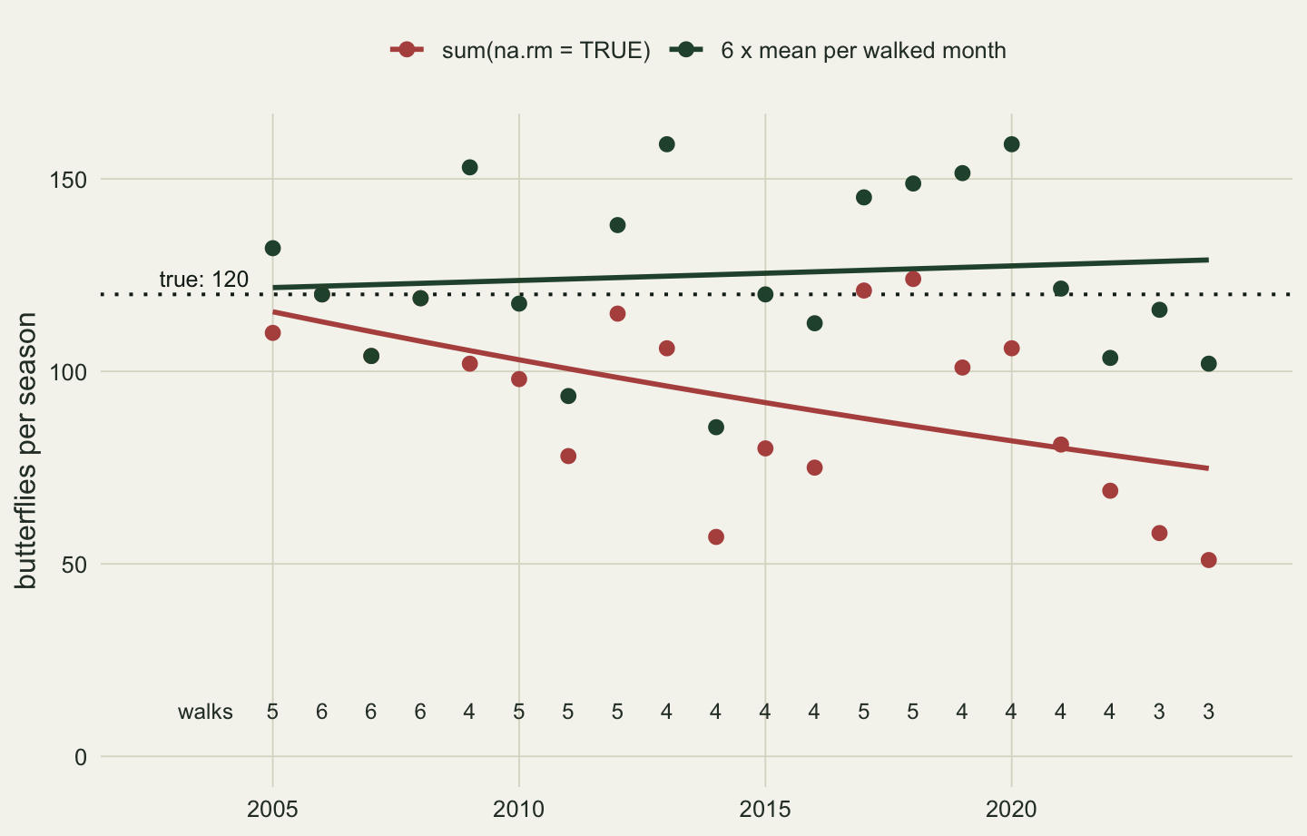
-20.4 27.0 18.0 A Poisson GLM of the yearly totals on year, the log-linear trend also fitted in Estimating population trends in R, reports a change of -20.4 per cent per decade. The population was built not to change. The first five seasons had 27 walks between them and the last five had 18.
Where the decline comes from
The decline can be worked out without a simulation. A month that is walked contributes its expected count to the total, and a month that is missed contributes 0. If each month is missed with probability p, the expected na.rm total is
expected total = (8 + 16 + 28 + 32 + 24 + 12) x (1 - p) = 120 x (1 - p)so it falls from 120 x 0.95 = 114 in 2005 to 120 x 0.60 = 72 in 2024 while the population stays at 120. The trend in the totals is the trend in 1 - p, the share of months walked. Fitting the same log-linear model to these expected totals gives the trend the naive analysis is aiming at (the chunk uses the quasipoisson family, because the expected totals are not whole numbers; the slope is the same as with poisson). The chunk then repeats the simulated transect 2000 times to check it:
expected_total <- 120 * (1 - p_missed)
closed_slope   <- coef(glm(expected_total ~ years, family = quasipoisson))[["years"]]
stopifnot(isTRUE(all.equal(closed_slope,                # same slope as poisson
  suppressWarnings(coef(glm(expected_total ~ years, family = poisson)))[["years"]])))

trend_pair <- function(counts) {
  total  <- rowSums(counts, na.rm = TRUE)
  walked <- rowSums(!is.na(counts))
  keep   <- walked > 0                                 # a year with no walks is unknown
  month  <- factor(rep(months, each = length(years)), levels = months)
  c(naive  = coef(glm(total ~ years, family = poisson))[["years"]],
    offset = coef(glm(total[keep] ~ years[keep] + offset(log(walked[keep])),
                      family = poisson))[[2]],
    month  = coef(glm(as.vector(counts) ~ rep(years, 6) + month,
                      family = poisson))[[2]],
    zero_years = sum(walked == 0))
}

set.seed(2016)
n_rep <- 2000
reps  <- t(replicate(n_rep, trend_pair(simulate_transect())))

naive_mean  <- mean(reps[, "naive"])
naive_mcse  <- sd(reps[, "naive"]) / sqrt(n_rep)
naive_neg   <- mean(reps[, "naive"] < 0)
naive_neg_se <- sqrt(naive_neg * (1 - naive_neg) / n_rep)
zero_share  <- mean(reps[, "zero_years"] > 0)
zero_expect <- sum(p_missed^6)                         # expected all-missed years per series
zero_prob   <- 1 - prod(1 - p_missed^6)                # chance of at least one such year
round(c(closed_per_decade = per_decade(closed_slope),
        sim_per_decade = per_decade(naive_mean),
        slope_gap_in_mcse = (naive_mean - closed_slope) / naive_mcse,
        share_negative = naive_neg, mcse = naive_neg_se,
        series_with_a_zero_year = zero_share, expected_zero_years = zero_expect,
        chance_of_a_zero_year = zero_prob), 4)
closed_per_decade sim_per_decade slope_gap_in_mcse
-21.2265 -21.4050 -0.9812
share_negative mcse series_with_a_zero_year
0.9905 0.0022 0.0120
expected_zero_years chance_of_a_zero_year
0.0148 0.0148 The expected totals give -21.2 per cent per decade. Across the 2000 simulated transects the average naive slope converts to -21.4 per cent per decade, 1.0 Monte Carlo standard errors from the worked-out value, and 99.1 per cent of the transects show a decline (Monte Carlo standard error 0.2 percentage points). The simulation adds nothing the arithmetic did not already say: a total with na.rm = TRUE measures butterflies counted, and here the butterflies counted per season went down because the walks went down.
A year with all six months missed is where the rule from the first section shows up on a plot. Its expected number per transect is the sum of p to the sixth power over the twenty years, 0.0148. The chance of at least one such year is 1 minus the product of (1 - p^6), 0.0148 (almost the same number, because the terms are tiny), and in the simulation 1.2 per cent of the 2000 transects had at least one such year (Monte Carlo standard error 0.2 percentage points). Each of those years went into the trend as a total of 0 butterflies: the lowest point on the graph, and the least informative one. The chance of an empty year is p to the power of the number of planned visits, so false zeros are rare with six visits and common with few: at the 2024 missed share of 40 per cent a year with three planned visits would be empty with probability 0.064, against 0.0041 with six.
Two fixes, measured with the same trend
The first fix is a different summary: the mean count per walked month, rowMeans(counts, na.rm = TRUE), which is the per_walk column above. Multiplied by 6 it is an estimate of the season total that does not shrink when walks are missed, and a year without walks comes out as NaN, so glm() drops it instead of fitting a zero.
The second fix is the model. Put the monthly counts in a long table, one row per month and year, and fit the Poisson GLM to them. glm() drops rows with a missing response by default (the na.action option is na.omit), so the unwalked months are simply absent, and a year with no walks has no rows. No offset is needed at the month level, because every row is one walk. If you keep the yearly table instead, the same model is the yearly total with offset(log(walked)), which turns the total into a rate per walk; Offsets for rates and densities in Poisson GLMs explains offsets. The two give the same slope to the last digit, which the chunk checks:
long <- data.frame(year  = rep(years, times = 6),
                   month = factor(rep(months, each = length(years)), levels = months),
                   count = as.vector(counts))
fit_month  <- glm(count ~ year, family = poisson, data = long)
fit_offset <- glm(total ~ year + offset(log(walked)), family = poisson,
                  data = yearly[yearly$walked > 0, ])

stopifnot(identical(getOption("na.action"), "na.omit"),
          is.nan(rowMeans(rbind(no_walks), na.rm = TRUE)),               # empty year: NaN
          length(fitted(glm(c(1, 2, NaN, 4) ~ seq_len(4), family = poisson))) == 3,
          length(fitted(fit_month)) == sum(!is.na(long$count)),   # missing rows dropped
          isTRUE(all.equal(coef(fit_month)[["year"]], coef(fit_offset)[["year"]],
                           tolerance = 1e-6)))
month_decade <- per_decade(coef(fit_month)[["year"]])

offset_mean   <- mean(reps[, "offset"])
offset_mcse   <- sd(reps[, "offset"]) / sqrt(n_rep)
offset_neg    <- mean(reps[, "offset"] < 0)
offset_neg_se <- sqrt(offset_neg * (1 - offset_neg) / n_rep)
month_mean_slope <- mean(reps[, "month"])
month_mcse    <- sd(reps[, "month"]) / sqrt(n_rep)
slope_sd      <- 10 * 100 * apply(reps[, c("offset", "month")], 2, sd)   # spread across transects
round(c(this_transect = month_decade,
        sim_per_decade = per_decade(offset_mean),
        mcse_per_decade = 10 * 100 * offset_mcse,
        share_negative = offset_neg, mcse = offset_neg_se,
        month_term_per_decade = per_decade(month_mean_slope),
        month_term_mcse = 10 * 100 * month_mcse,
        sd_without_month = slope_sd[["offset"]], sd_with_month = slope_sd[["month"]]), 4)
this_transect sim_per_decade mcse_per_decade
3.0607 -0.1594 0.1223
share_negative mcse month_term_per_decade
0.5080 0.0112 -0.0976
month_term_mcse sd_without_month sd_with_month
0.0916 5.4688 4.0974 On the transect above the monthly model gives +3.1 per cent per decade, against -20.4 from the na.rm totals. Across the 2000 transects the average slope converts to -0.16 per cent per decade (Monte Carlo standard error about 0.12), and 50.8 per cent of the transects show a decline (Monte Carlo standard error 1.1), which is what a population with no trend should give: half up, half down. Adding a term for the month, count ~ year + month, does no harm here: its average slope over the same 2000 transects converts to -0.10 per cent per decade (Monte Carlo standard error about 0.09), and the slopes of single transects spread less (standard deviation 4.1 against 5.5 per cent per decade without it), because a year that happens to miss July no longer looks poorer than one that misses April. It is also the version that survives the next section.
When some months are missed more than others
Both fixes rest on one assumption: once the year is known, a month is missed for reasons that have nothing to do with how many butterflies it would have had. In the simulation above that is true by construction: the chance of a missed walk depends on the year and on nothing else. That is not “missing completely at random” in the sense of Missing data: MCAR, MAR and MNAR, because the chance changes with the year; it is missing at random given the year, and a summary or a model that takes the year into account, as both fixes do, is not biased by it. Nakagawa and Freckleton (2008) set out why ecologists should say which case they are in before they drop anything.
Suppose instead that the volunteers who drop out stop walking at the edges of the season. The next chunk keeps the same share of missed months each year but puts every missed walk in April, May or September, the three months with the lowest expected counts, each missed with twice the yearly probability:
edge_months <- c("Apr", "May", "Sep")
p_edge <- matrix(0, length(years), 6, dimnames = list(years, months))
p_edge[, edge_months] <- 2 * p_missed                 # same expected share missed per year
stopifnot(isTRUE(all.equal(rowMeans(p_edge), p_missed, check.attributes = FALSE)))

trend_edge <- function(counts) {
  long <- data.frame(year  = rep(years, times = 6),
                     month = factor(rep(months, each = length(years)), levels = months),
                     count = as.vector(counts))
  c(naive       = coef(glm(rowSums(counts, na.rm = TRUE) ~ years, family = poisson))[["years"]],
    per_walk    = coef(glm(count ~ year, family = poisson, data = long))[["year"]],
    month_term  = coef(glm(count ~ year + month, family = poisson, data = long))[["year"]])
}

set.seed(2017)
reps_edge <- t(replicate(n_rep, trend_edge(simulate_transect(p_edge))))
edge_decade <- per_decade(colMeans(reps_edge))
edge_mcse   <- 10 * 100 * apply(reps_edge, 2, sd) / sqrt(n_rep)
edge_up     <- mean(reps_edge[, "per_walk"] > 0)
round(rbind(per_decade = edge_decade, mcse = edge_mcse), 2)
naive per_walk month_term
per_decade -11.92 11.90 0.07
mcse 0.12 0.11 0.09c(share_per_walk_rising = edge_up)share_per_walk_rising
0.992 Now the naive total falls by 11.9 per cent per decade, less than before, because the months being lost are the ones that held few butterflies. The mean per walked month goes wrong the other way: the months still walked are increasingly the rich midsummer ones, and the monthly GLM without a month term reports +11.9 per cent per decade, an increase in 99 per cent of the transects. Here the reason for missing a walk is the month, and the month is recorded, so it can go into the model: count ~ year + month compares each month with itself across years and gives +0.07 per cent per decade. In the terms of Rubin (1976) this is still missing at random, now given the year and the month, so the model needs both. Butterfly monitoring schemes take the same route with more machinery: a model of the seasonal pattern, fitted to the counts that were made, gives an index of abundance that allows for missing counts (Rothery and Roy 2001). If walks were missed because of the weather on days with few butterflies, and the weather was not recorded, neither fix could correct it from these counts alone.
What to check in your own data
Before any na.rm = TRUE, count the missing values per group: rowSums(is.na(counts)) or table(year, is.na(count)). If that count changes over the years, a sum with na.rm = TRUE will change with it.
Keep the number of visits in the yearly table next to every total, and plot it under the series, as the figure above does. A reader who sees the visits thinning out will ask the right question. A rate per walk is only as good as the walk: it assumes a walk in 2024 is the same effort as a walk in 2005. In casual records, where visits get longer and recorders choose where to go, it is not, and Reporting rates and effort drift measures the false trend that leaves in a per-list rate.
Search your script for sum( and rowSums( with na.rm = TRUE and ask of each one whether a missing value means “nobody looked” or “looked and found none”. Only the second is a zero. For the first, use a mean per visit or a model of the visit-level counts.
Look for zeros in your yearly totals and check each against the number of visits. A zero from a year with no visits should be NA, and it should not reach a trend model.
If visits were missed more in some months or sites than others, put that month or site in the model (as count ~ year + month), and say in the methods why visits were missed, as far as you know.
References
Nakagawa S, Freckleton RP 2008 Trends in Ecology and Evolution 23(11):592-596 (10.1016/j.tree.2008.06.014)
Rothery P, Roy DB 2001 Journal of Applied Statistics 28(7):897-909 (10.1080/02664760120074979)
Rubin DB 1976 Biometrika 63(3):581-592 (10.1093/biomet/63.3.581)