library(ggplot2)
library(classInt)

te_paper  <- "#f5f4ee"; te_ink    <- "#16241d"; te_body   <- "#2c3a31"
te_forest <- "#275139"; te_rust   <- "#b5534e"; te_gold   <- "#c9b458"
te_line   <- "#dad9ca"

theme_datasheet <- function() {
  theme_minimal(base_size = 12) +
    theme(plot.background  = element_rect(fill = te_paper, colour = NA),
          panel.background = element_rect(fill = te_paper, colour = NA),
          panel.grid.major = element_line(colour = te_line, linewidth = 0.3),
          panel.grid.minor = element_blank(),
          text             = element_text(colour = te_body),
          plot.title       = element_text(colour = te_ink, face = "bold"),
          plot.subtitle    = element_text(colour = te_body),
          axis.text        = element_text(colour = te_body))
}
class_ver <- as.character(packageVersion("classInt"))Natural breaks in QGIS and R: Jenks on large layers
R
QGIS
GIS
spatial
classInt
cartography
ecology tutorial
QGIS Natural Breaks against R classInt on a species richness grid: which modes match exactly, and why Jenks above 30009 cells classifies phantom zeros.
A stacked species distribution model has given you predicted species richness on a one kilometre grid, 300 cells wide and 200 tall, and you want two versions of the same map: a quick one in QGIS to look at, and the figure for the paper drawn in R. In QGIS you open Layer > Layer Properties > Symbology, pick Graduated, set Mode to Natural Breaks (Jenks) and press Classify. In R you call classInt::classIntervals(style = "jenks"). Both claim to do the same thing, which is to cut the values into classes that are as internally homogeneous as possible, and on this grid they do not return the same classes.
Mapping species richness in R with sf builds a richness grid and hands it to QGIS as a GeoPackage for styling; this post is about the first styling decision after that handoff. Choosing colours for ecological data is about which colours go on the map; the question here is which values each colour is given to. And where Running QGIS from the command line compares Processing algorithms with sf and terra, classification is not a Processing algorithm at all: qgis_process has nothing called Jenks, so the QGIS side below is PyQGIS, calling the same renderer code the Symbology dialog calls. The exact algorithm for one variable is Fisher’s (1958), and Jenks and Caspall (1971) framed the choice of classes on a choropleth map as an error to be made as small as possible. What follows is not a new method but a check of two implementations of it against each other.
No chunk on this page calls QGIS, because the page has to build on a machine that does not have it. The R chunks write the input files, a Python script ran once against QGIS 3.34.4-Prizren on Linux and wrote its class tables as small CSV files next to this page, and the R chunks read those files back. The script is qgis-classes.py, in the same folder.
The grid, and the files QGIS read
Richness is built from a regional gradient, three hotspots and cell noise, so the bulk of the cells sit in the high teens and twenties and a long tail runs up to the hotspot cores, the right skewed shape for which Natural Breaks is usually chosen. A second column holds the change in richness between two periods, which runs from losses to gains. The chunk writes the grid in shuffled row order, so that the first n rows of the file are a random n cells of the map, and it writes a ten kilometre version, the mean of each ten by ten block.
set.seed(20261012)
n_col <- 300; n_row <- 200
cells <- expand.grid(col = seq_len(n_col), row = seq_len(n_row))
bump  <- function(cx, cy, s, a) a * exp(-((cells$col - cx)^2 + (cells$row - cy)^2) / (2 * s^2))
cells$richness <- 16 + 0.04 * cells$row + bump(70, 140, 18, 55) + bump(210, 60, 25, 40) +
  bump(250, 160, 10, 70) + rnorm(nrow(cells), 0, 3)
cells$change <- -8 + 0.08 * cells$row + bump(210, 60, 25, -6) + rnorm(nrow(cells), 0, 2.5)
cells$richness <- round(cells$richness, 4); cells$change <- round(cells$change, 4)
write.csv(cells[sample(nrow(cells)), ], "richness-1km.csv", row.names = FALSE)
blk <- interaction((cells$col - 1) %/% 10, (cells$row - 1) %/% 10, drop = TRUE)
write.csv(data.frame(col = tapply((cells$col - 1) %/% 10 + 1, blk, `[`, 1),
                     row = tapply((cells$row - 1) %/% 10 + 1, blk, `[`, 1),
                     richness = round(tapply(cells$richness, blk, mean), 4)),
          "richness-10km.csv", row.names = FALSE)
grid_1km  <- read.csv("richness-1km.csv"); grid_10km <- read.csv("richness-10km.csv")
qgis_in   <- read.csv("qgis-input-check.csv")
same_input <- qgis_in$cells_1km == nrow(grid_1km) && qgis_in$cells_10km == nrow(grid_10km) &&
  isTRUE(all.equal(c(qgis_in$sum_10km, qgis_in$sum_richness, qgis_in$sum_change),
                   c(sum(grid_10km$richness), sum(grid_1km$richness), sum(grid_1km$change)),
                   tolerance = 1e-10))
rich_q <- quantile(grid_1km$richness, c(0.5, 0.99))
The one kilometre grid has 60000 cells with predicted richness from 5.0 to 97.0, a median of 22.3 and a 99th percentile of 68.4; the ten kilometre grid has 600. The QGIS script recorded how many rows it read from each file and the sum of each column, and comparing those with what R reads here returns TRUE. If you rebuild this page and that says FALSE, the class tables below were computed from a different file and the comparisons stop meaning anything.
Four modes on a small layer
On the ten kilometre grid every QGIS mode works on all 600 values, with no sampling anywhere. The PyQGIS part is short: build a point layer from the CSV and ask each classification class for five classes. The upper bounds go to qgis-10km-breaks.csv.
for mode, cls in [("equal", QgsClassificationEqualInterval), ("quantile", QgsClassificationQuantile),
                  ("jenks", QgsClassificationJenks), ("pretty", QgsClassificationPrettyBreaks)]:
    for i, c in enumerate(cls().classes(lay10, "v", 5)):
        out.append(dict(mode=mode, klass=i + 1, lower=repr(bounds(c)[0]), upper=repr(bounds(c)[1])))
q10 <- read.csv("qgis-10km-breaks.csv"); v10 <- grid_10km$richness
qup <- function(m) q10$upper[q10$mode == m]
r_equal <- classIntervals(v10, 5, style = "equal")$brks[-1]
r_quant <- quantile(v10, (1:5) / 5, type = 7, names = FALSE)
other_ty <- sapply(c(1:6, 8:9), function(ty)
max(abs(quantile(v10, (1:5) / 5, type = ty, names = FALSE) - qup("quantile"))))
r_jenks <- classIntervals(v10, 5, style = "jenks")$brks[-1]
r_fisher <- classIntervals(v10, 5, style = "fisher")
r_pretty <- classIntervals(v10, 5, style = "pretty")$brks[-1]
q_pretty <- qup("pretty")
fmt <- function(z) paste(sprintf("%.4f", z), collapse = ", ")
mode_tab <- data.frame(
qgis_mode = c("Equal Interval", "Equal Count (Quantile)", "Natural Breaks (Jenks)",
"Pretty Breaks"),
r_call = c('`classIntervals(style = "equal")`', "`quantile(type = 7)`",
'`classIntervals(style = "jenks")`', '`classIntervals(style = "pretty")`'),
qgis_upper = c(fmt(qup("equal")), fmt(qup("quantile")), fmt(qup("jenks")), fmt(q_pretty)),
r_upper = c(fmt(r_equal), fmt(r_quant), fmt(r_jenks), fmt(r_pretty)),
identical = c(identical(qup("equal"), r_equal), identical(qup("quantile"), r_quant),
identical(qup("jenks"), r_jenks), identical(q_pretty, r_pretty)))
knitr::kable(mode_tab, col.names = c("QGIS mode", "R call", "QGIS upper bounds",
"R upper bounds", "identical"),
caption = "Five classes asked for, ten kilometre grid, upper bound of each class.")| QGIS mode | R call | QGIS upper bounds | R upper bounds | identical |
|---|---|---|---|---|
| Equal Interval | classIntervals(style = "equal") |
27.7735, 39.8101, 51.8466, 63.8832, 75.9197 | 27.7735, 39.8101, 51.8466, 63.8832, 75.9197 | FALSE |
| Equal Count (Quantile) | quantile(type = 7) |
18.6207, 21.3722, 23.2521, 27.6863, 75.9197 | 18.6207, 21.3722, 23.2521, 27.6863, 75.9197 | TRUE |
| Natural Breaks (Jenks) | classIntervals(style = "jenks") |
20.7135, 27.1160, 37.6361, 51.3886, 75.9197 | 20.7995, 27.1160, 37.6361, 51.3886, 75.9197 | FALSE |
| Pretty Breaks | classIntervals(style = "pretty") |
20.0000, 30.0000, 40.0000, 50.0000, 60.0000, 70.0000, 75.9197 | 20.0000, 30.0000, 40.0000, 50.0000, 60.0000, 70.0000, 80.0000 | FALSE |
n_pretty_q <- length(q_pretty); n_pretty_r <- length(r_pretty)
inner_same <- all(head(q_pretty, -1) == head(r_pretty, -1))
jenks_gap  <- max(abs(qup("jenks") - r_jenks)); jenks_ndiff <- sum(qup("jenks") != r_jenks)
Equal Interval and Quantile are the same formulas in both programs: on this layer identical() on the vectors of doubles is TRUE for both. That is exact here, not a guarantee to the last bit on every layer, because QGIS adds the equal interval step repeatedly where R multiplies it, and it computes the quantile position in a slightly different order; any difference sits in the last bits of a double, far below anything a legend prints. The QGIS quantile is R’s type 7, the default of quantile(); the other eight types miss it by between 0.0337 and 0.0680 richness units. (The comment above that code in qgsclassificationquantile.cpp describes an (n + 1) rule, which would be type 6; the line underneath it computes q * (n - 1), which is type 7.) Pretty Breaks agree on every interior break, and both returned 7 classes when asked for five, because a pretty sequence picks the round step first and lets the class count follow. They differ only at the ends: R’s classes run from 10 to 80, while QGIS starts the first class at the data minimum and stops the last at the data maximum, 75.9197. That the interior breaks are equal as doubles is TRUE.
Natural Breaks does not match: of the five upper bounds, 1 differs, the lowest, by 0.0860, and the other four agree.
Where the Jenks difference comes from
classInt and QGIS run the same dynamic programming algorithm, and the QGIS source names the classInt code as one of its bases. The algorithm fills a table, row by row, with the cheapest way to split the first l sorted values into j classes, remembering where the last class starts, and then walks back through that table from the top. The difference is in the walk back. classInt stores the position where the last class starts and steps back to the value before it. QGIS stores the position of the last value before the start, then subtracts one more:
            matrixOne[l][j] = i4;
...
    k = matrixOne[k][j] - 1;
Those are lines 171 and 188 of qgsclassificationjenks.cpp on the 3.34 branch. The break it reports at each step is still a real class boundary, but the next step looks up the best split of one value fewer than it should, so the classes below it come from a different problem, whose answer can be far from the best one. With two classes the walk back takes only one step and the extra subtraction is never used, so only three or more classes are affected. The chunk below ports that function to R line by line, vectorising only the innermost loop, with a switch that removes the extra - 1.
qgis_jenks <- function(smp, k, fix = FALSE) {
  smp <- sort(smp); n <- length(smp)
  one <- matrix(0L, n + 1, k); two <- matrix(0, n + 1, k)   # row l + 1 holds l values
  one[1:2, ] <- 1L; two[3:(n + 1), ] <- .Machine$double.xmax
  for (l in 2:n) {
    vals <- smp[l:1]                         # the inner loop visits values l, l - 1, ..., 1
    s1 <- cumsum(vals); s2 <- cumsum(vals * vals); w <- seq_len(l)
    v  <- s2 - s1 * s1 / w                   # sum of squares of the last w values
    i4 <- l - w; ok <- i4 != 0
    for (j in 2:k) {
      cand <- v[ok] + two[i4[ok] + 1, j - 1]
      best <- max(which(cand == min(cand)))  # QGIS tests >=, so the last minimum wins
      one[l + 1, j] <- i4[ok][best]; two[l + 1, j] <- cand[best]
    }
    one[l + 1, 1] <- 1L; two[l + 1, 1] <- v[l]
  }
  brk <- numeric(k); brk[k] <- smp[n]; kk <- n
  for (j in k:2) {
    brk[j - 1] <- smp[one[kk + 1, j]]
    kk <- if (fix) one[kk + 1, j] else one[kk + 1, j] - 1
  }
  brk
}
# which class QGIS draws a value in: the first range with lower <= value <= upper
qgis_class <- function(x, lower, upper) {
  cl <- rep(NA_integer_, length(x))
  for (k in seq_along(lower)) cl[is.na(cl) & x >= lower[k] & x <= upper[k]] <- k
  cl
}
gvf <- function(x, cl) 1 - sum(tapply(x, cl, function(z) sum((z - mean(z))^2))) /
  sum((x - mean(x))^2)
port_same  <- identical(qgis_jenks(v10, 5), qup("jenks"))
fixed_same <- identical(qgis_jenks(v10, 5, fix = TRUE), r_jenks)
cl_q10  <- qgis_class(v10, q10$lower[q10$mode == "jenks"], qup("jenks"))
cl_r10  <- findInterval(v10, r_jenks[-5], left.open = TRUE) + 1
cl_f10  <- findCols(r_fisher)
moved   <- sum(cl_q10 != cl_r10); fisher_part <- identical(cl_f10, as.integer(cl_r10))
gvf_q10 <- gvf(v10, cl_q10); gvf_r10 <- gvf(v10, cl_r10)
The port reproduces the QGIS breaks exactly (identical() gives TRUE), and with the extra step removed it reproduces classInt exactly (TRUE). On this layer the cost is small: 7 of 600 cells change class, and the goodness of variance fit, one minus the within class sum of squares over the total sum of squares, is 0.947481 for QGIS against 0.947484 for the optimum. style = "fisher" in classInt finds the same partition as style = "jenks": that the two put every cell in the same class is TRUE. It reports the breaks differently, as midpoints between the last value of one class and the first of the next, so its first break prints as 20.8093 where jenks prints 20.7995. For a legend that difference is cosmetic; for reproducing someone’s classes it is not.
Seven values with an obvious answer
On the ten kilometre grid the extra step moved one break a little. Seven values show what it can do. The values 1, 2, 3, 50, 100, 101 and 102 fall into three groups that anyone would draw, and the script classed them through the same Graduated renderer call as before, into two and into three classes, and wrote the ranges to qgis-tiny.csv:
tiny = [1, 2, 3, 50, 100, 101, 102]
for k in [2, 3]:
    ranges, tally = graduated_jenks(point_layer(tiny_rows, "v", len(tiny)), k)
qt <- read.csv("qgis-tiny.csv"); x7 <- c(1, 2, 3, 50, 100, 101, 102)
q7_3 <- qt[qt$k == 3, ]; q7_2 <- qt[qt$k == 2, ]
wss <- function(x, lower, upper) # within class sum of squares
sum(tapply(x, qgis_class(x, lower, upper), function(z) sum((z - mean(z))^2)))
up7 <- list(qgis = q7_3$upper, port = qgis_jenks(x7, 3), fixed = qgis_jenks(x7, 3, fix = TRUE),
jenks = classIntervals(x7, 3, style = "jenks")$brks[-1])
tiny_tab <- data.frame(
route = c("QGIS, Graduated renderer (`qgis-tiny.csv`)", "R port of the QGIS function",
"R port without the extra step", '`classIntervals(style = "jenks")`'),
upper = sapply(up7, function(u) paste(u, collapse = ", ")),
sizes = sapply(up7, function(u) paste(tabulate(qgis_class(x7, c(min(x7), head(u, -1)), u), 3),
collapse = ", ")),
wss = sapply(up7, function(u) sprintf("%.1f", wss(x7, c(min(x7), head(u, -1)), u))))
knitr::kable(tiny_tab, row.names = FALSE,
col.names = c("route", "upper bounds", "values per class", "within class SS"),
caption = "Three classes of the seven values 1, 2, 3, 50, 100, 101, 102.")| route | upper bounds | values per class | within class SS |
|---|---|---|---|
QGIS, Graduated renderer (qgis-tiny.csv) |
1, 50, 102 | 1, 3, 3 | 1506.7 |
| R port of the QGIS function | 1, 50, 102 | 1, 3, 3 | 1506.7 |
| R port without the extra step | 3, 50, 102 | 3, 1, 3 | 4.0 |
classIntervals(style = "jenks") |
3, 50, 102 | 3, 1, 3 | 4.0 |
tiny_port <- identical(up7$port, up7$qgis); tiny_opt <- identical(up7$fixed, up7$jenks)
two_same  <- identical(q7_2$upper, classIntervals(x7, 2, style = "jenks")$brks[-1])
QGIS puts 1 alone in the first class and 2 and 3 in a class with 50. Its first class runs from 1 to 1 and holds 1 value, and its within class sum of squares is 1506.7 against 4.0 for the obvious grouping. The port gives the QGIS answer (TRUE), and without the extra step it gives the classInt answer (TRUE). With two classes, where the step is never used, QGIS and classInt agree: TRUE.
How often does this matter on a layer small enough that QGIS uses every value? The chunk below draws 200 right skewed (lognormal) layers of each of three sizes, classes each into five with the port as it stands and with the extra step removed, and records how often the two disagree and what the QGIS classes lose in goodness of variance fit.
set.seed(20261012)
cls_up <- function(x, up) findInterval(x, head(up, -1), left.open = TRUE) + 1
small <- do.call(rbind, lapply(c(30, 100, 400), function(n) {
  r <- replicate(200, {
    x <- rlnorm(n, 0, 1); a <- qgis_jenks(x, 5); b <- qgis_jenks(x, 5, fix = TRUE)
    c(differ = !identical(a, b), loss = gvf(x, cls_up(x, b)) - gvf(x, cls_up(x, a)))
  })
  data.frame(n = n, differ = mean(r["differ", ]), med_loss = median(r["loss", r["differ", ] == 1]),
             max_loss = max(r["loss", ]))
}))
knitr::kable(small, digits = c(0, 3, 4, 3),
             col.names = c("values", "share with different classes", "median GVF loss, when different",
                           "largest GVF loss"),
caption = "Five classes on 200 lognormal layers of each size: QGIS against the optimum.")| values | share with different classes | median GVF loss, when different | largest GVF loss |
|---|---|---|---|
| 30 | 0.735 | 0.0038 | 0.183 |
| 100 | 0.770 | 0.0009 | 0.090 |
| 400 | 0.810 | 0.0002 | 0.030 |
At every size the QGIS classes differ from the optimum in most layers, in 74 to 81 per cent of them. The loss is usually small: among the layers where the classes differ, the median loss in goodness of variance fit is 0.0038 at 30 values and less on larger layers. The worst cases are not small. On layers of 30 values the largest loss was 0.183, and on layers of 400 it was still 0.030. So the step matters on small layers too, where QGIS uses every value and no sampling can be blamed.
Above 3000 cells, QGIS classifies a sample
The algorithm costs time in proportion to the square of the number of values, so QGIS does not run it on a large layer. The header sets mMaximumSize = 3000, and above that the function builds a sample instead. Since QGIS 3.20 the sample is systematic: sort all values, put the minimum and maximum in the first two slots, and step through the sorted values so that 2998 more of them, evenly spaced in rank, fill the next slots. That makes the classes stable from one click to the next, which the earlier random sample was not, and it is also what the port needs to reproduce QGIS on the full grid.
qgis_sample <- function(x, max_size = 3000) {
  n_val <- length(x); s <- sort(x)
  if (n_val <= max_size) return(s)
  out <- numeric(max(max_size, n_val %/% 10))    # sample.resize(max(3000, n / 10))
  out[1] <- min(x); out[2] <- max(x)
  i <- 1:(n_val - 3); step <- (i * (max_size - 2)) %/% (n_val - 2)
  pick <- i[step > c(-1, head(step, -1))]         # j++ whenever the integer ratio moves on
  out[2 + seq_along(pick)] <- s[pick + 1]
  out
}
runs <- read.csv("qgis-jenks-runs.csv")
run_id <- unique(runs[, c("field", "n", "shift")])
run_id$zeros <- NA_integer_; run_id$port_same <- NA
run_id$gvf <- NA_real_; run_id$first_share <- NA_real_; run_id$first_upper <- NA_real_
for (r in seq_len(nrow(run_id))) {
  sel <- runs$field == run_id$field[r] & runs$n == run_id$n[r] & runs$shift == run_id$shift[r]
  x   <- grid_1km[[run_id$field[r]]][seq_len(run_id$n[r])] + run_id$shift[r]
  smp <- qgis_sample(x)
  run_id$zeros[r]     <- sum(smp == 0)          # the richness values are all above zero
  run_id$port_same[r] <- identical(qgis_jenks(smp, 5), runs$upper[sel])
  run_id$gvf[r]         <- gvf(x, qgis_class(x, runs$lower[sel], runs$upper[sel]))
  run_id$first_share[r] <- runs$features[sel][1] / run_id$n[r]
  run_id$first_upper[r] <- runs$upper[sel][1]
}
all_port <- all(run_id$port_same); n_runs <- nrow(run_id)
rich <- run_id[run_id$field == "richness" & run_id$shift == 0, ]
opt_gvf <- function(x, k = 5) {
  ci <- classIntervals(x, k, style = "fisher", largeN = Inf, warnLargeN = FALSE)
  gvf(x, findCols(ci))
}
n_check <- c(5000, 20000, 30009)
gvf_gap <- sapply(n_check, function(n) opt_gvf(grid_1km$richness[1:n]) - rich$gvf[rich$n == n])
For every one of the 27 QGIS runs in qgis-jenks-runs.csv, from 1000 to 60000 cells, the R port applied to this reconstructed sample returns exactly the doubles QGIS wrote: that all of them are identical is TRUE. Up to 30009 cells the sample costs very little on this layer. At 5000, 20000 and 30009 cells the QGIS classes fall short of the best possible fit on all cells by \(4.5 \times 10^{-7}\), \(6.8 \times 10^{-6}\) and \(7.8 \times 10^{-6}\) in goodness of variance fit. This smooth richness surface forgives a sample of 3000 ranks. A layer with a long upper tail may fare worse, since a rank sample keeps only a few of its extreme cells; that was not tested here.
Above 30009 cells, the sample holds zeros
The sample array is sized as the larger of 3000 and one tenth of the number of values, but the loop that fills it counts only to 3000. The comment above the resize says the intention: “sample at least maximumSize values or a 10% sample, whichever is larger”. The fill loop still computes its slot counter as i * (mMaximumSize - 2) / (sorted.size() - 2), which stays below mMaximumSize - 2, so once a tenth of the layer exceeds 3000, the slots beyond the first 3000 are never written, and a resized QVector<double> holds 0.0 in every slot it has not been given. Those zeros are then sorted in with the real values and classified as data. With integer division, n / 10 first exceeds 3000 at n = 30010, and from there the number of zeros is n / 10 - 3000.
z_pred <- function(n) pmax(0, n %/% 10 - 3000)
z_ok   <- all(rich$zeros == z_pred(rich$n))
first_z <- min(rich$n[rich$zeros > 0]); last_clean <- max(rich$n[rich$zeros == 0])
b_before <- runs$upper[runs$field == "richness" & runs$n == last_clean & runs$shift == 0][1]
b_after  <- runs$upper[runs$field == "richness" & runs$n == first_z & runs$shift == 0][1]
smp_z <- qgis_sample(grid_1km$richness[seq_len(first_z)])
b_nozero <- qgis_jenks(smp_z[smp_z != 0], 5)[1]         # the same sample with its one zero taken out
collapse_n <- min(rich$n[rich$first_share < 0.01]); held_n <- max(rich$n[rich$first_share >= 0.01])
r60 <- rich[rich$n == 60000, ]
q60 <- runs[runs$field == "richness" & runs$n == 60000 & runs$shift == 0, ]
x60 <- grid_1km$richness
t_fisher <- system.time(ci_opt <- classIntervals(x60, 5, style = "fisher", largeN = Inf))[["elapsed"]]
opt60 <- gvf(x60, findCols(ci_opt)); opt60_4 <- opt_gvf(x60, 4)
opt_upper <- sort(attr(ci_opt, "parameters")[, "max"])
The count of zeros in the reconstructed sample matches n / 10 - 3000 at every grid size: TRUE. The first run with any zero is at 30010 cells, and QGIS’s own output moves there: the first break is 20.7751 at 30009 cells and 20.7453 at 30010, a shift that the port reproduces with its single zero. Without that one zero the port returns 20.7750 at 30010 cells, next to the 20.7751 at 30009. A handful of zeros only nudges the lowest class. By 30500 cells (50 zeros) the classes have reorganised: the first class is now the block of zeros plus the lowest few real cells, and at 30200 cells it had not yet. On the full grid of 60000 cells half of the sample, 3000 of 6000 values, is zeros that are not in the layer. The legend’s first class runs from 4.996 to 8.693 and holds 42 cells, 0.07 per cent of the map, while the remaining four classes share everything else from breaks computed on the 3000 real values.
smp60 <- sort(qgis_sample(x60))
ggplot(data.frame(pos = seq_along(smp60), val = smp60,
                  kind = ifelse(seq_along(smp60) <= z_pred(60000), "padding zero", "sampled value")),
       aes(pos, val, colour = kind)) +
  geom_hline(yintercept = min(x60), linetype = "dashed", colour = te_body, linewidth = 0.4) +
  geom_point(size = 0.4) +
  scale_x_continuous(breaks = c(1, 1500, 3000, 4500, 6000)) +
  scale_colour_manual(values = c("padding zero" = te_rust, "sampled value" = te_forest), name = NULL) +
  labs(x = "position in the sorted sample", y = "value classified (richness)",
       title = "What Natural Breaks classifies at 60000 cells",
       subtitle = "dashed line: the smallest richness in the layer") +
  theme_datasheet() + theme(legend.position = "bottom") +
  guides(colour = guide_legend(override.aes = list(size = 2.5)))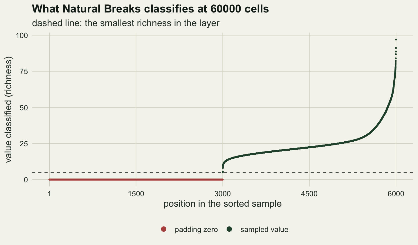
The goodness of variance fit tells you what the wasted class costs. On all 60000 cells the QGIS classes reach 0.8942. The best five classes reach 0.9276, and the best four reach 0.8936. The QGIS fit sits a little above the best four classes and far below the best five: on a large layer of positive values, Natural Breaks in QGIS gives you, in effect, four classes and a legend entry.
brk_long <- runs[runs$field == "richness" & runs$shift == 0 & runs$klass < 5, ]
brk_long$break_no <- factor(paste("break", brk_long$klass))
ggplot(brk_long, aes(n, upper, colour = break_no)) +
  geom_hline(yintercept = opt_upper[1:4], colour = "#b9b8a6", linewidth = 0.7) +
  geom_vline(xintercept = c(3000, 30010), linetype = "dashed", colour = te_body, linewidth = 0.4) +
  geom_line(linewidth = 0.7) + geom_point(size = 1.8) +
  scale_x_log10(breaks = c(1000, 3000, 10000, 30010, 60000),
                labels = c("1000", "3000", "10000", "30010", "60000")) +
  scale_colour_manual(values = c(te_forest, te_gold, te_rust, "#7f8c84"), name = NULL) +
  labs(x = "cells classified (log scale)", y = "upper bound of class (richness)",
       title = "Stable until the zeros arrive",
       subtitle = "QGIS Natural Breaks, first n cells of the 1 km grid") +
  theme_datasheet() + theme(legend.position = "bottom")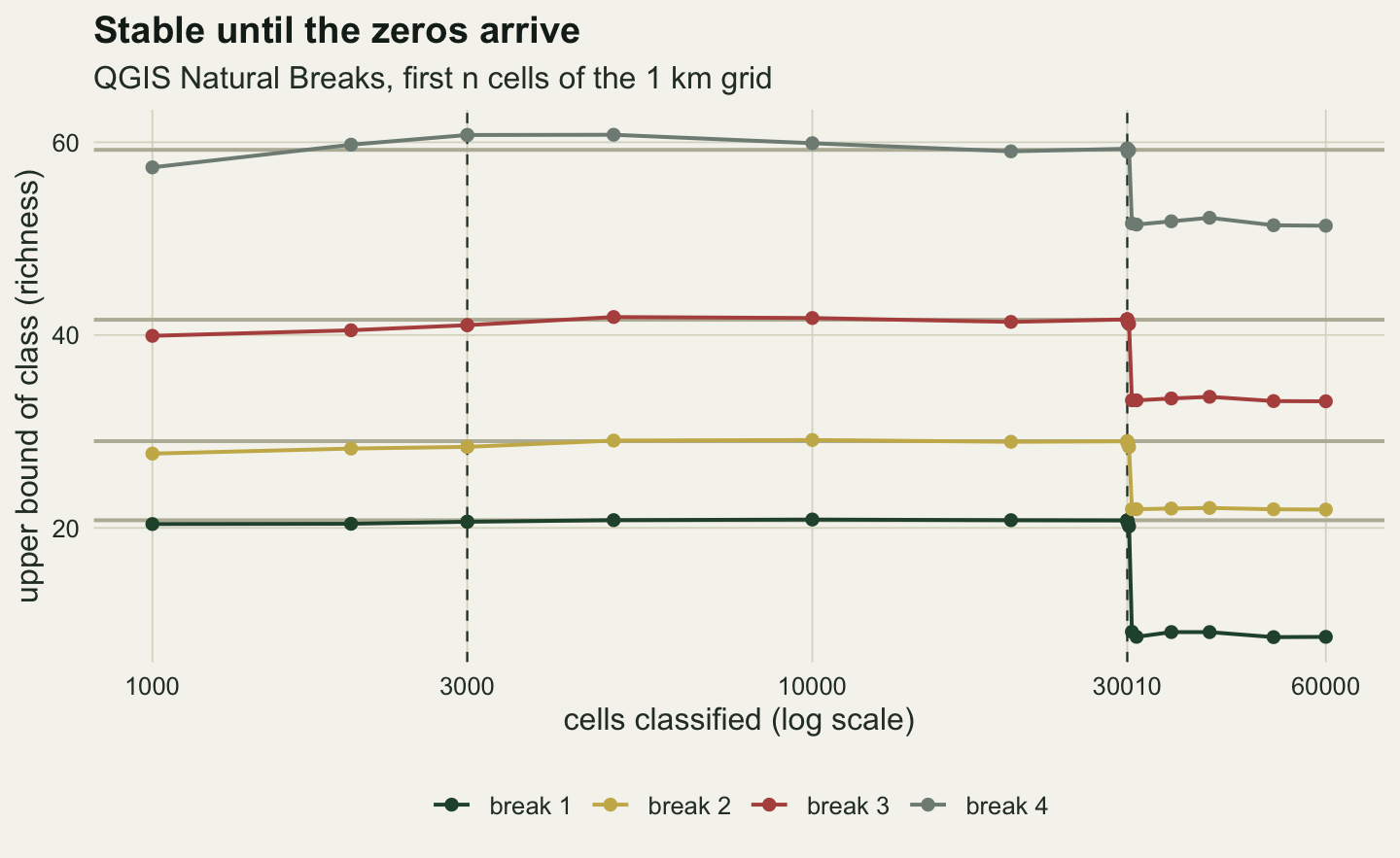
How far the data sit from zero decides what the legend shows
The zeros are always at zero, and what they do depends on where the data are. On this grid the smallest richness is close enough to zero that the zeros take a few real cells with them into the first class. The script also classified the full grid with a constant added to every cell, as if the same map came from a richer region.
sh <- run_id[run_id$field == "richness" & run_id$n == 60000, ]
sh$min_value <- min(x60) + sh$shift
q_sh <- runs[runs$field == "richness" & runs$n == 60000, ]
sh$first_lower <- q_sh$lower[q_sh$klass == 1]
sh$first_count <- q_sh$features[q_sh$klass == 1]
knitr::kable(sh[, c("shift", "min_value", "first_lower", "first_upper", "first_count", "gvf")],
             row.names = FALSE, digits = c(1, 3, 3, 3, 0, 4),
             col.names = c("added", "layer minimum", "class 1 from", "class 1 to",
                           "cells in class 1", "GVF"),
caption = "QGIS Natural Breaks on all 60000 cells, with a constant added.")| added | layer minimum | class 1 from | class 1 to | cells in class 1 | GVF |
|---|---|---|---|---|---|
| 0.0 | 4.996 | 4.996 | 8.693 | 42 | 0.8942 |
| 2.5 | 7.496 | 7.496 | 8.005 | 2 | 0.8936 |
| 5.0 | 9.996 | 9.996 | 10.505 | 2 | 0.8936 |
| 10.0 | 14.996 | 14.996 | 0.000 | 0 | 0.8936 |
| 20.0 | 24.996 | 24.996 | 0.000 | 0 | 0.8936 |
| 40.0 | 44.996 | 44.996 | 0.000 | 0 | 0.8936 |
inv <- sh[sh$first_upper < sh$first_lower, ]With 10.0 or more added, the first class becomes the pure form of the defect: it runs from the layer minimum, 14.996, down to 0.0, an upper bound below its lower bound, and no cell can fall in it. QGIS puts that line in the legend with a colour and draws four colours on the map. The second class then starts at zero, so it silently takes in everything from the layer minimum up to its own upper bound. On a layer that crosses zero, such as the change in richness between two periods, the zeros land inside the range instead.
xc <- grid_1km$change
qc <- runs[runs$field == "change" & runs$n == 60000, ]
gvf_c  <- run_id$gvf[run_id$field == "change" & run_id$n == 60000]
ci_c   <- classIntervals(xc, 5, style = "fisher", largeN = Inf)
gvf_co <- gvf(xc, findCols(ci_c)); up_co <- sort(attr(ci_c, "parameters")[, "max"])
shift_c <- qc$upper[1:4] - up_co[1:4]
neg_share <- mean(xc < 0)
smp_c <- qgis_sample(xc); real_c <- head(smp_c, 3000)    # the 3000 slots the fill loop writes
dev_c <- rbind(qgis_jenks(smp_c, 5), qgis_jenks(smp_c, 5, fix = TRUE),
               qgis_jenks(real_c, 5), qgis_jenks(real_c, 5, fix = TRUE))[, 1:4] -
  matrix(up_co[1:4], 4, 4, byrow = TRUE)
knitr::kable(data.frame(sample = c("with the zeros", "with the zeros", "without the zeros",
                                   "without the zeros"),
                        walk_back = c("QGIS", "extra step removed", "QGIS", "extra step removed"),
                        dev_c), digits = 3, row.names = FALSE,
             col.names = c("sample", "walk back", "break 1", "break 2", "break 3", "break 4"),
caption = "Change layer, 60000 cells: each interior break minus the optimal break on all cells.")| sample | walk back | break 1 | break 2 | break 3 | break 4 |
|---|---|---|---|---|---|
| with the zeros | QGIS | 0.065 | 0.184 | 0.196 | 0.110 |
| with the zeros | extra step removed | 0.076 | 0.188 | 0.196 | 0.110 |
| without the zeros | QGIS | -0.040 | -0.016 | -0.008 | 0.005 |
| without the zeros | extra step removed | -0.032 | -0.016 | -0.002 | 0.005 |
51 per cent of the change values are losses, and the middle class straddles zero in both classifications: QGIS puts its breaks at -6.5249, -2.1683, 1.9776, 6.0598, the optimum on all cells at -6.5903, -2.3522, 1.7817, 5.9500. Each QGIS interior break lies between 0.065 and 0.196 above the optimal one. The table takes that shift apart by running the port on the same sample with and without its zeros, with and without the extra step. Almost all of it comes from the zeros. Without them, and with the QGIS walk back kept, every break is within 0.040 of the optimum; with the zeros kept and the extra step removed, the breaks still lie between 0.076 and 0.196 above it. On a spread this wide the fit hardly changes: the goodness of variance fit is 0.94116 against 0.94124. A layer with a narrower spread around zero, or with a real spike of zeros such as a count of individuals, is where padding inside the range would matter more, and it is not measured here.
The same fill loop is in every branch checked on 2026-09-25: 3.20, 3.22, 3.28, 3.34, 3.40, 3.44 and master. Up to 3.18 every slot after the first two, the extra ones included, was filled with a random draw, so there were no zeros, but the classes changed at every click (GitHub issue 31723 reported exactly that); the change to a systematic sample removed the randomness and left the extra slots empty. The Symbology dialog reaches this function directly. Classify in the Graduated widget (qgsgraduatedsymbolrendererwidget.cpp) calls the renderer’s updateClasses(), which calls the method’s classes() on the whole layer, which calls calculateBreaks() in qgsclassificationjenks.cpp; the script above goes through the same updateClasses() call. The dialog does have a warning for Natural Breaks on more than 50000 features, but it only appears when the method reports a complexity above 1, and PyQGIS reports 1 for QgsClassificationJenks, so it never appears. We searched the QGIS issue trackers (GitHub and the older Redmine) and found no report of the padding zeros. For the backtracking step there is a possible one: issue 28299 (QGIS 3.4, opened in 2018 and still open) reports a Natural Breaks first class holding a single value and the other classes wrong, which is what the extra step does to the seven values above, and the same two lines were already in the 3.4 code. The issue gives no diagnosis, and we could not download its data to run them again, so the match is in the symptom only. We reported both defects to the QGIS project on 25 September 2026 as issue 67546, together with a third one in the same function: when a layer has no more features than classes, the function returns the values in feature order, unsorted, so the legend shows overlapping and inverted ranges.
cl_opt <- qgis_class(x60, c(min(x60), head(opt_upper, -1)), opt_upper)
cl_q60 <- qgis_class(x60, q60$lower, q60$upper)
class_tab <- function(lower, upper, cl)
  data.frame(range = sprintf("%.3f to %.3f", lower, upper), cells = tabulate(cl, 5))
opt_lower <- c(min(x60), head(opt_upper, -1))
leg_opt <- class_tab(opt_lower, opt_upper, cl_opt); leg_q <- class_tab(q60$lower, q60$upper, cl_q60)
knitr::kable(data.frame(class = 1:5, leg_opt, leg_q), row.names = FALSE,
             col.names = c("class", "optimal, all cells (R)", "cells", "Natural Breaks (QGIS)", "cells"),
caption = "The two legends for the full grid, with the number of cells drawn in each class.")| class | optimal, all cells (R) | cells | Natural Breaks (QGIS) | cells |
|---|---|---|---|---|
| 1 | 4.996 to 20.791 | 23060 | 4.996 to 8.693 | 42 |
| 2 | 20.791 to 28.995 | 25133 | 8.693 to 21.896 | 28037 |
| 3 | 28.995 to 41.590 | 6714 | 21.896 to 33.127 | 23375 |
| 4 | 41.590 to 59.212 | 3814 | 33.127 to 51.341 | 5904 |
| 5 | 59.212 to 97.005 | 1279 | 51.341 to 97.005 | 2642 |
ramp <- c("1" = "#efe7c2", "2" = "#a9c08a", "3" = "#5d8a5e", "4" = te_forest, "5" = te_ink)
maps <- rbind(data.frame(grid_1km[, c("col", "row")], how = "optimal breaks, all cells (R)",
                         cls = factor(cl_opt, levels = 1:5)),
              data.frame(grid_1km[, c("col", "row")], how = "Natural Breaks (QGIS)",
                         cls = factor(cl_q60, levels = 1:5)))
maps$how <- factor(maps$how, levels = unique(maps$how))
ggplot(maps, aes(col, row, fill = cls)) + geom_raster() +
  facet_wrap(~ how, ncol = 2) + coord_fixed(expand = FALSE) +
  scale_fill_manual(values = ramp, drop = FALSE, name = "class") +
  labs(x = NULL, y = NULL) + theme_datasheet() +
  theme(axis.text = element_blank(), panel.grid.major = element_blank(),
        strip.text = element_text(colour = te_ink, face = "bold", size = 11),
        legend.position = "bottom")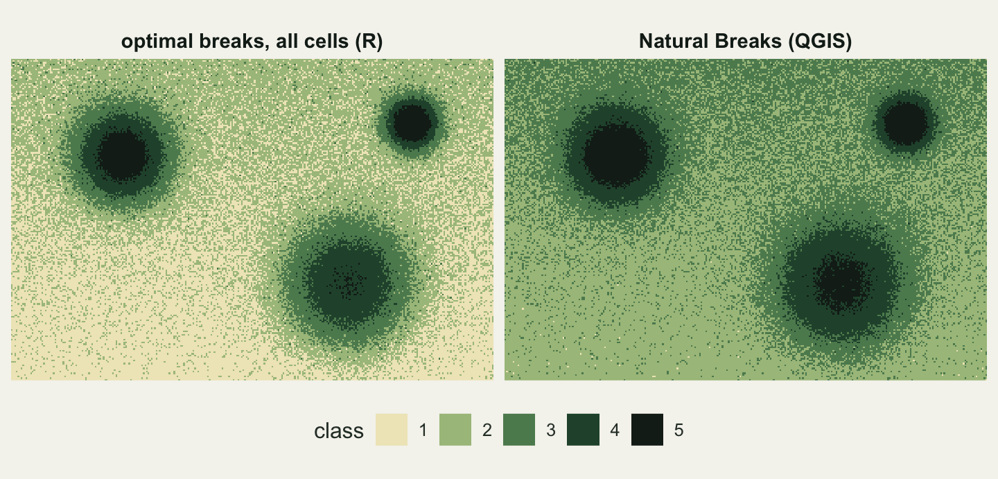
On the map the missing class is easy to miss. The palest colour is still in the legend, attached to 42 cells that the eye cannot find, so the background that the optimum draws in the two palest colours is drawn one step darker, and the rings round the hotspots widen: the third class holds 23375 cells in QGIS against 6714 in the optimum. Anyone reading the legend sees five classes and has no reason to count them.
R samples too, at random
classInt has the same problem of cost and solves it differently. For style = "fisher" and style = "jenks" only, and only while warnLargeN = TRUE (the default), when the number of distinct values is above largeN (default 3000), it warns and classifies the minimum and maximum plus a random sample of the values, as many as a tenth of the distinct values, capped at largeN. There is no padding, but without a seed the breaks change from one call to the next.
set.seed(1)
r_def <- t(replicate(20, suppressWarnings(classIntervals(x60, 5, style = "fisher"))$brks[2:5]))
r_gvf <- apply(r_def, 1, function(b) gvf(x60, findInterval(x60, b) + 1))
n_distinct <- length(unique(x60)); n_draw <- min(ceiling(0.1 * n_distinct), 3000)
t_j <- sapply(c(600, 1500), function(n) system.time(
  classIntervals(grid_1km$richness[1:n], 5, style = "jenks"))[["elapsed"]])
jenks_60k_min <- t_j[2] * (60000 / 1500)^2 / 60
The grid has 52585 distinct values, so each call draws 3000 of them. Over 20 calls in a row the top break ranged from 55.60 to 63.05 and the lowest from 20.25 to 21.45, around optimal values of 59.21 and 20.79. The fit barely suffers, 0.9261 to 0.9276 against 0.9276, but a figure redrawn tomorrow will have a different legend. Two fixes work. largeN = Inf runs Fisher’s algorithm on every value: it took 7.1 seconds for all 60000 cells on the machine that built this page, which is a price worth paying once. It is not a fix for style = "jenks", which is written in plain R loops: it took 0.24 seconds for 600 values and 1.69 for 1500, and scaling the second by the square of the size puts the full grid at about 45 minutes. The other fix is to keep the sample and set a seed, which makes the figure reproducible without making it optimal. Silencing the warning is not a third fix: warnLargeN = FALSE also turns the sampling off, so the full computation runs, which for style = "jenks" means the plain R loop on every cell estimated above; use style = "fisher". Note that R counts distinct values: a richness grid of whole species counts has far fewer than 3000 distinct values, so R never samples it, while QGIS counts features and pads it all the same.
rows3 <- rbind(data.frame(route = "optimal, all cells", b = opt_upper[1:4]),
               data.frame(route = "R default sampling", b = as.vector(r_def)),
               data.frame(route = "QGIS Natural Breaks", b = q60$upper[1:4]))
rows3$route <- factor(rows3$route, levels = rev(unique(rows3$route)))
ggplot(rows3, aes(b, route, colour = route)) +
  geom_point(data = rows3[rows3$route != "R default sampling", ], size = 2.8) +
  geom_point(data = rows3[rows3$route == "R default sampling", ], size = 2.4, alpha = 0.75,
             position = position_jitter(height = 0.12, width = 0, seed = 3)) +
  scale_colour_manual(values = c("optimal, all cells" = te_forest, "R default sampling" = te_gold,
                                 "QGIS Natural Breaks" = te_rust), guide = "none") +
  scale_y_discrete(limits = levels(rows3$route)) +
  labs(x = "interior break (richness)", y = NULL, title = "Three routes to Natural Breaks, 60000 cells") +
  theme_datasheet()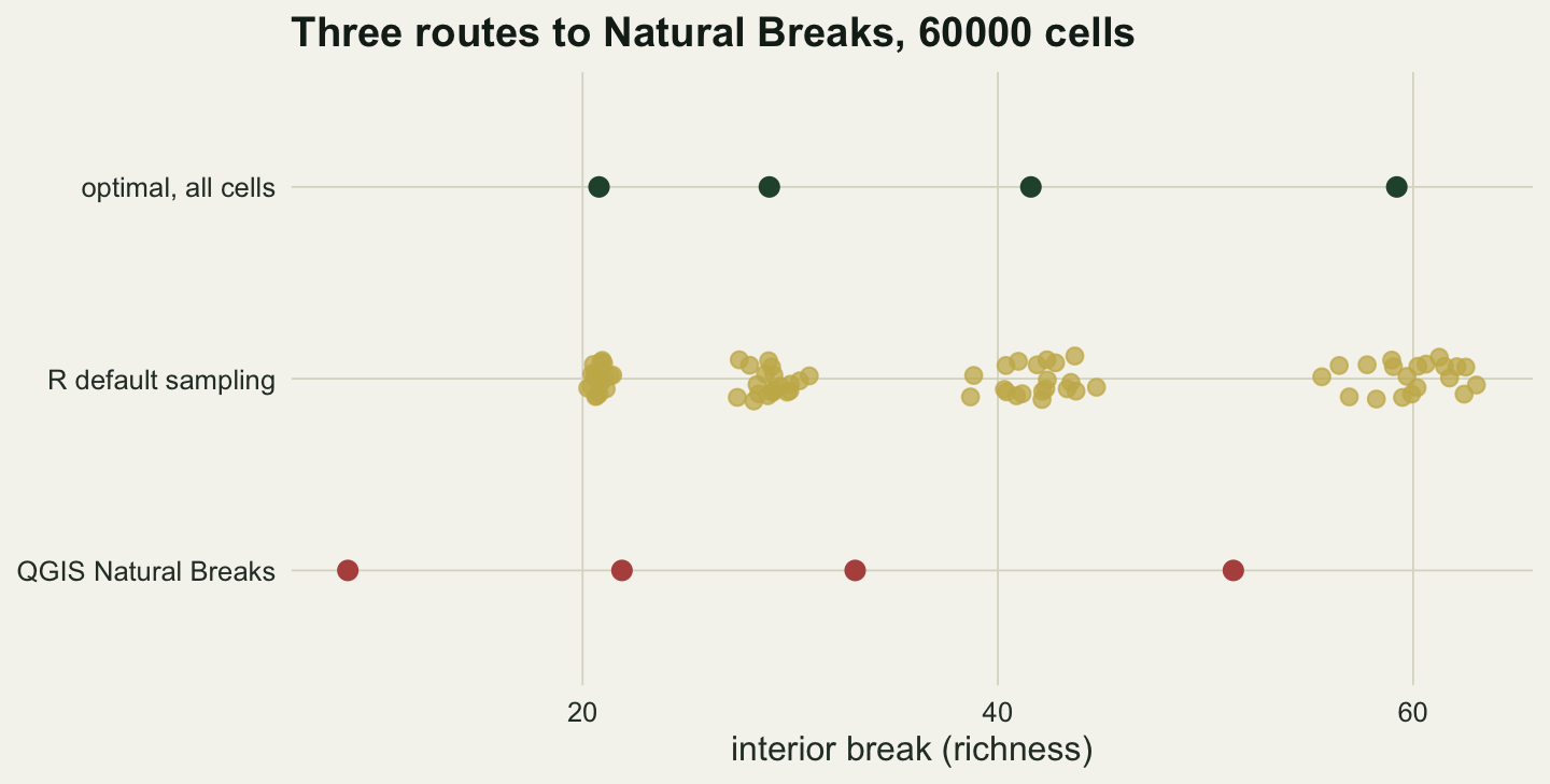
What to report, and what to do
For a map in a paper, compute the breaks where you can see them. In R that is classIntervals(x, 5, style = "fisher", largeN = Inf) on every value, or sort(attr(ci, "parameters")[, "max"]) on its result ci if you want breaks that are data values rather than midpoints. If the map is finished in QGIS, type those numbers in: in the Classes tab of the Graduated renderer, set the number of classes first, then double click a value range and enter the bounds, so that QGIS never runs its own classification. Changing the number of classes, or the Mode, afterwards recomputes the classes and overwrites the typed values. Equal Interval and Equal Count (Quantile) are safe alternatives on any size of layer, because they do not sample and use the same formulas as R. Natural Breaks in QGIS needs the same care at any size. On layers of up to 3000 features it uses every value, but the backtracking step can still move classes (the seven values above, and most of the small skewed layers in the table), so for a published map compute the breaks in R and type them in whatever the layer size. On a larger layer also look twice at the legend: an upper bound below its lower bound, or a first class holding a handful of features, is the padding. In a methods section, say which algorithm, on how many values, with which software version, and whether the classes were computed on all values or on a sample. “Natural Breaks (Jenks) in QGIS” on 60000 cells means classes from 3000 values and 3000 zeros.
Honest limits
Everything here is one synthetic layer and one QGIS build, 3.34.4 on Linux. The other branches were checked by reading the source, not by running them; the fill loop and the walk back are unchanged in 3.40, 3.44 and master, but a later release may fix either. The size of each effect depends on the data: the cost of the rank sample was small on this smooth surface, the cost of the backtracking step was small here and on most of the small lognormal layers but large on a few of them, and the padding produced a near empty class here, an inverted empty class once the data sat far enough from zero, and only a small shift in breaks on the change layer. None of those magnitudes transfers to another layer; the mechanism does. The Symbology dialog itself was never clicked, because this QGIS runs headless: the claim that it uses the same code rests on the widget source and on the script calling the same renderer method. Reading the loop further, its index product i * (mMaximumSize - 2) is computed in 32 bit integers and overflows on layers of more than about 716000 features; what the compiled code does on layers that large was not tested. Goodness of variance fit is one criterion for a classification, and a cartographer may prefer classes that fit worse and read better.
References
Fisher WD 1958 Journal of the American Statistical Association 53(284):789-798 (10.1080/01621459.1958.10501479)
Jenks GF, Caspall FC 1971 Annals of the Association of American Geographers 61(2):217-244 (10.1111/j.1467-8306.1971.tb00779.x)
Bivand R 2023 classInt: Choose Univariate Class Intervals. R package version 0.4-10 (https://CRAN.R-project.org/package=classInt)