library(sf)
library(lwgeom)
library(ggplot2)

te_paper  <- "#f5f4ee"; te_ink    <- "#16241d"; te_body   <- "#2c3a31"
te_forest <- "#275139"; te_rust   <- "#b5534e"; te_gold   <- "#c9b458"
te_line   <- "#dad9ca"

theme_datasheet <- function() {
  theme_minimal(base_size = 12) +
    theme(plot.background  = element_rect(fill = te_paper, colour = NA),
          panel.background = element_rect(fill = te_paper, colour = NA),
          panel.grid.major = element_line(colour = te_line, linewidth = 0.3),
          panel.grid.minor = element_blank(),
          text             = element_text(colour = te_body),
          plot.title       = element_text(colour = te_ink, face = "bold"),
          plot.subtitle    = element_text(colour = te_body),
          axis.text        = element_text(colour = te_body))
}

soft <- sf_extSoftVersion()
sf_ver <- as.character(packageVersion("sf")); lw_ver <- as.character(packageVersion("lwgeom"))
proj_r <- unname(soft["PROJ"]); geos_r <- unname(soft["GEOS"])
qgis_ver <- "3.34.4"; proj_q <- "9.4.0" # from qgis_process --version, where the files were madeArea in QGIS and R: which call matches which
R
QGIS
sf
GIS
spatial
ecology tutorial
QGIS $area, area() and sf st_area() give different areas for one habitat patch. Each has an exact partner in the other tool, and headless QGIS hides a trap.
Three habitat patches have been digitised in QGIS: a pond complex, a beech wood and a block of hay meadows. The obvious next step is an area column. The field calculator offers two ways to get one, $area and area($geometry), and the Add geometry attributes tool offers three more. Then the layer goes to R and st_area() produces yet another number. They do not all agree to the square metre, and on some layers they do not agree to the hectare. The question is which one is right, and which call in one program gives the same number as which call in the other.
Choosing a projection for area and distance has already measured how far apart those answers can be inside sf: the s2 sphere against the ellipsoid, the small gap between two sensible projections, and Web Mercator more than doubling an area. That post stays in R and is not repeated here. This one is the other half of the job. For each area that QGIS can hand you, it names the one line of R that reproduces it, and it shows the two project settings that decide what $area returns: the ellipsoid and the area unit. The desktop fills both in for you. The command line runner leaves them empty, and then $area quietly returns a flat area in the layer’s own units, which on a longitude and latitude layer means square degrees.
The page has no screenshots. Menu paths are given in bold, and the QGIS numbers come from small files in this post’s folder, produced by the commands shown in plain fenced blocks. No chunk on this page calls QGIS: the page is built on a machine that runs R only, so the QGIS half is a transcript, as in Running QGIS from the command line. If you have never moved a layer between the two programs, From QGIS to R: a spatial join with GeoPackage is the gentler start.
The short answer
For a table of patch areas, the number you usually want is the area on the WGS 84 ellipsoid. In the QGIS desktop that is what $area gives, provided Project > Properties > General shows WGS 84 as the ellipsoid and square metres as the Units for area measurements, both in the Measurements frame. In R the same number comes from lwgeom::st_geod_area(x), or from st_area(x) after sf_use_s2(FALSE), with x in longitude and latitude; transform a projected layer with st_transform(x, 4326) first, because on a projected layer st_area() returns the flat area. Plain st_area(x) on a longitude and latitude layer measures on a sphere instead; at the latitude of these patches that comes out a little smaller, and the sign of the gap changes with latitude. area($geometry) in QGIS is a flat area in the layer’s own units, and its partner is st_area() on the same projected layer. When QGIS runs from the command line with qgis_process, pass --ELLIPSOID=EPSG:7030 (WGS 84) or a saved project with --PROJECT_PATH; without either, $area is the flat area.
The full correspondence, with x a longitude and latitude layer:
| In QGIS | Partner in R (sf, lwgeom) |
What the number is |
|---|---|---|
$area, project ellipsoid WGS 84, area unit square metres |
st_geod_area(x), or st_area(x) after sf_use_s2(FALSE) |
square metres on the ellipsoid |
$area, the same project with area unit hectares |
st_geod_area(x) / 1e4 |
hectares on the ellipsoid |
$area, project ellipsoid Krassowsky 1940 |
st_geod_area() with the Krassowsky ellipsoid attached |
square metres on that ellipsoid |
$area, custom sphere of radius 6371010 m |
st_area(x), the default with s2 on |
square metres on a sphere |
area($geometry) on a projected layer |
st_area() on the same projected layer |
flat square metres of that projection |
area($geometry) on a longitude and latitude layer |
st_area(st_set_crs(x, NA)) |
square degrees |
$area, project ellipsoid None / Planimetric |
st_area(st_set_crs(x, NA)) * 12392029030.5 on lon/lat, st_area() if projected |
flat area, labelled square metres |
$area in qgis_process with no ellipsoid and no project |
the same as area($geometry) |
flat area in the layer’s units |
Every row is measured below on three patches, and the last measured section gives the largest gap for each pair.
Three patches, in three coordinate systems
The patches are synthetic and illustrative: smooth three lobed outlines placed near 46.77 N, 23.59 E, built in longitude and latitude with radii set in kilometres. The chunk writes the same three patches three times, as GeoPackages in longitude and latitude (EPSG:4326), in UTM zone 34 north (EPSG:32634) and in Web Mercator (EPSG:3857). Those three files are the input to every QGIS command below. A layer arriving in Web Mercator is not a contrived case: it is what you get from many web map services and from anything digitised on top of a tile basemap without a change of CRS.
lon0 <- 23.59; lat0 <- 46.77; km_deg <- 111.32   # window centre; rule of thumb km per degree
blob <- function(cx, cy, r_km) {                 # a three lobed outline, 40 vertices
  th <- seq(0, 2 * pi, length.out = 41)[-41]
  rr <- r_km * (1 + 0.2 * sin(3 * th))
  m  <- cbind(cx + rr / (km_deg * cos(cy * pi / 180)) * cos(th), cy + rr / km_deg * sin(th))
  st_polygon(list(rbind(m, m[1, ])))
}
patches <- st_sf(patch = c("pond complex", "beech wood", "hay meadows"),
  geometry = st_sfc(blob(lon0 - 0.3, lat0 - 0.1, 0.5), blob(lon0, lat0, 1),
                    blob(lon0 + 0.2, lat0 + 0.1, 2), crs = 4326))
layer_crs <- c(4326, 32634, 3857)
layers <- lapply(layer_crs, function(code) {
  out <- if (code == 4326) patches else st_transform(patches, code)
  st_write(out, sprintf("patches-%d.gpkg", code), delete_dsn = TRUE, quiet = TRUE)
  st_read(sprintf("patches-%d.gpkg", code), quiet = TRUE)
})
names(layers) <- c("lonlat", "utm", "mercator")
Seven area columns from the field calculator
In the desktop, the field calculator lives behind Layer > Open Attribute Table, as the abacus button in the table’s toolbar (Ctrl+I), and in the Processing toolbox as Vector table > Field calculator. The toolbox version is native:fieldcalculator, and that is what the loop below runs, once per new column. Each column is the same expression or a close relative, computed with a different setting: area($geometry); $area with no ellipsoid given; $area with the WGS 84 ellipsoid (EPSG:7030); $area on a sphere of radius 6371010 metres; and $area inside three saved projects, one whose CRS is the Romanian Stereo70 system (EPSG:3844), one set to None / Planimetric and one on WGS 84 with its area unit set to hectares. The three project files are made by the PyQGIS script in the section on the desktop default further down.
export QT_QPA_PLATFORM=offscreen
add() {  # input, output, new field name, expression, then any extra flags
  qgis_process run native:fieldcalculator "${@:5}" -- INPUT="$1" OUTPUT="$2" \
    FIELD_NAME="$3" FIELD_TYPE=0 FIELD_LENGTH=0 FIELD_PRECISION=0 FORMULA="$4" > /dev/null
}
for crs in 4326 32634 3857; do
  add patches-$crs.gpkg s1.gpkg planar 'area($geometry)'
  add s1.gpkg s2.gpkg no_ellipsoid '$area'
  add s2.gpkg s3.gpkg wgs84 '$area' --ELLIPSOID=EPSG:7030
  add s3.gpkg s4.gpkg sphere '$area' --ELLIPSOID=PARAMETER:6371010:6371010
  add s4.gpkg s5.gpkg stereo70_project '$area' --PROJECT_PATH=stereo70.qgs
  add s5.gpkg s6.gpkg planimetric_project '$area' --PROJECT_PATH=planimetric.qgs
  add s6.gpkg qgis-area-$crs.csv hectares_project '$area' --PROJECT_PATH=hectares.qgs
  rm s?.gpkg
done
The chunk below reads the three files back and sets the three main QGIS columns next to their R partners, patch by patch.
read_q <- function(code) read.csv(sprintf("qgis-area-%d.csv", code))
q_ll <- read_q(4326); q_utm <- read_q(32634); q_merc <- read_q(3857)
a_ell <- as.numeric(st_geod_area(patches))           # WGS 84 ellipsoid
a_s2  <- as.numeric(st_area(patches))                # sf default, s2 on
a_utm <- as.numeric(st_area(layers$utm))             # flat, UTM 34N
m2 <- function(v) sprintf("%.2f", v)
side_by_side <- data.frame(patch = q_ll$patch,
  q_wgs = m2(q_ll$wgs84), r_ell = m2(a_ell), q_sph = m2(q_ll$sphere), r_s2 = m2(a_s2),
  q_utm = m2(q_utm$planar), r_utm = m2(a_utm))
knitr::kable(side_by_side, align = "lrrrrrr",
  col.names = c("patch", "QGIS `$area`, WGS 84", "`st_geod_area(x)`", "QGIS `$area`, sphere",
                "`st_area(x)`", "QGIS `area($geometry)`, UTM", "`st_area(x_utm)`"),
caption = "Square metres, QGIS columns read from qgis-area-4326.csv and qgis-area-32634.csv.")| patch | QGIS $area, WGS 84 |
st_geod_area(x) |
QGIS $area, sphere |
st_area(x) |
QGIS area($geometry), UTM |
st_area(x_utm) |
|---|---|---|---|---|---|---|
| pond complex | 796406.07 | 796406.07 | 794325.26 | 794325.26 | 796369.67 | 796369.67 |
| beech wood | 3185698.68 | 3185698.68 | 3177300.89 | 3177300.89 | 3186212.56 | 3186212.56 |
| hay meadows | 12743091.63 | 12743091.63 | 12709202.25 | 12709202.25 | 12747059.67 | 12747059.67 |
Each QGIS column and the R column to its right agree in every printed digit. The sections below take the pairs one at a time.
$area is ellipsoidal, and so is sf with s2 switched off
With an ellipsoid set, $area is the area of the polygon on that ellipsoid, with its edges taken as geodesics, the shortest paths on the ellipsoid. In sf, a longitude and latitude layer is measured on the ellipsoid only when spherical geometry is switched off; st_area() then hands the job to lwgeom::st_geod_area(), which can also be called directly.
sf_use_s2(FALSE); a_off <- as.numeric(st_area(patches)); sf_use_s2(TRUE)
route_same <- identical(a_ell, a_off)
gap_ell    <- max(abs(q_ll$wgs84 - a_ell)); rel_ell <- max(abs(q_ll$wgs84 - a_ell) / a_ell)
gap_ell_pr <- max(abs(c(q_utm$wgs84, q_merc$wgs84) - rep(a_ell, 2)))
km2 <- a_ell / 1e6
The two R routes return identical values (identical() is TRUE), and they match the QGIS wgs84 column to within 25.808 square millimetres, on patches of 0.80, 3.19 and 12.74 square kilometres. That is not two good algorithms happening to agree. It is one algorithm: both programs hand the polygon to the same routine inside PROJ, Karney’s (2013) method for the area of a geodesic polygon. The few square millimetres left over are, relative to areas of that size, floating-point rounding in double precision arithmetic, not a difference of method.
The wgs84 columns of the UTM and Web Mercator files carry the same numbers, to within 78.515 square millimetres. With an ellipsoid set, QGIS first converts each vertex of a projected layer back to longitude and latitude and then measures on the ellipsoid, so the CRS of the layer stops mattering. That is the property you want from a measurement, and it is the reason $area in the desktop is usually the number to trust.
The sf default is a sphere
Leave s2 on, which has been the sf default since version 1.0 (Pebesma and Bivand 2023 explain the switch), and a longitude and latitude layer is measured on a sphere with a radius of 6371010 metres, the default radius of the s2 library. QGIS can measure on that sphere too: a custom ellipsoid whose two axes are equal is a sphere.
gap_s2  <- max(abs(q_ll$sphere - a_s2)); rel_s2 <- max(abs(q_ll$sphere - a_s2) / a_s2)
sph_pct <- 100 * (a_s2 / a_ell - 1)
n_empty <- sum(is.na(c(q_utm$sphere, q_merc$sphere)))
The QGIS sphere column and plain st_area() agree to within 1.334 square millimetres. That gap is larger than on the ellipsoid because two different routines are at work here, the s2 library’s own spherical area in R and the ellipsoidal routine with zero flattening in QGIS, but it is still a relative difference of at most \(3.2 \times 10^{-13}\), which closes the correspondence for the default sf call. The sphere sits 0.26 to 0.27 per cent below the ellipsoid on these patches. The projection post derives that gap from the two radii of curvature at this latitude, and it is not a disagreement between the programs: it is the difference between two surfaces.
One thing did not work. On the UTM and Web Mercator layers the same call returned not-a-number, which the GeoPackage in the loop stored as an empty field: 6 empty values out of 6, with no message. In QGIS 3.34 a custom ellipsoid comes without a longitude and latitude system to convert projected vertices into, so their coordinates in metres reach the area routine as if they were degrees. The 3.40 and 3.44 source adds that system (see the section on the source below), so projected layers should work there, but that was read, not run. On a longitude and latitude layer the sphere works in 3.34, and that is the only case where you would want it.
area($geometry) is flat, in the layer’s own units
area() ignores every ellipsoid setting. It is the planar area of the coordinates as they are stored, in the units of the layer’s CRS, and its partner in R is st_area() on the same projected layer. On a longitude and latitude layer the stored coordinates are degrees, so the result is in square degrees. sf has no default call that returns that, because it goes to s2 instead; you get it only by removing the CRS first.
a_merc <- as.numeric(st_area(layers$mercator))
a_deg  <- as.numeric(st_area(st_set_crs(patches, NA)))
gap_utm <- max(abs(q_utm$planar - a_utm)); gap_merc <- max(abs(q_merc$planar - a_merc))
gap_deg <- max(abs(q_ll$planar - a_deg))
utm_pct  <- 100 * (a_utm / a_ell - 1); merc_pct <- 100 * (a_merc / a_ell - 1)
deg_to_km2 <- a_ell / a_deg / 1e6                # km2 per square degree, patch by patch
All three pairs match: 2.973 square millimetres apart on the UTM layer, 5.472 on the Web Mercator layer, and equal to within floating-point rounding on the longitude and latitude layer, where the unit is the square degree. On the UTM layer the flat area is within 0.031 per cent of the ellipsoidal one, which is why nobody working in UTM notices the difference between area($geometry) and $area. On the Web Mercator layer it is 112 to 114 per cent too large, the inflation the projection post measured.
The square degree column is not an area in any useful sense. Here a square degree covers 8507 square kilometres at the southern patch and 8476 at the northern one, because a degree of longitude shrinks with latitude, so no single multiplier turns such a column into square metres. The next section shows QGIS applying one anyway.
Which ellipsoid and unit the desktop uses
So $area is only as good as the ellipsoid behind it, and the ellipsoid belongs to the project. It is shown and set in Project > Properties > General, in the Measurements frame, where the first choice in the list is None / Planimetric; the same frame holds the Units for area measurements, and $area is converted into that unit. The help text of $area says both: the result follows the project’s ellipsoid setting and its area unit.
A new desktop project gets an ellipsoid without anyone choosing one. With the default Settings > Options > CRS and Transforms > CRS Handling choice, Use CRS from first layer added, the first layer loaded sets the project CRS, and the project’s ellipsoid is set from that CRS too, unless the option Planimetric measurements on the same page is ticked. It ships unticked. Changing the CRS later in Project > Properties > CRS moves the ellipsoid along with it, unless the ellipsoid has been set to None / Planimetric. A new project starts with square metres as its area unit unless the options have been changed. The script below makes the same call the desktop makes for the three CRS of this page and for Stereo70, and records the ellipsoid each one leaves behind. It then saves the three project files the loop above reads, with the user name, author and save time removed.
import os, re
from qgis.core import (QgsApplication, QgsProject, QgsCoordinateReferenceSystem,
                       QgsProjectMetadata, Qgis)
app = QgsApplication([], False); app.initQgis()
project = QgsProject.instance()

def save(name):  # write a project file without the user name, author or save time
    project.setMetadata(QgsProjectMetadata())
    project.write(name)
    for extra in [name.replace(".qgs", "_attachments.zip"), name + "~"]:
        if os.path.exists(extra): os.remove(extra)   # side files, not needed
    text = open(name).read()
    text = re.sub(r' saveUser(Full)?="[^"]*"| saveDateTime="[^"]*"', "", text)
    open(name, "w").write(text)

rows = ["project_crs,ellipsoid"]
for code in ["EPSG:4326", "EPSG:32634", "EPSG:3857", "EPSG:3844"]:
    project.setCrs(QgsCoordinateReferenceSystem(code), True)  # as the desktop does
    rows.append(f"{code},{project.ellipsoid()}")
open("qgis-project-ellipsoid.csv", "w").write("\n".join(rows) + "\n")
save("stereo70.qgs")                       # the CRS set last: EPSG:3844

project.setCrs(QgsCoordinateReferenceSystem("EPSG:4326"), True)
project.setEllipsoid("NONE")               # Measurements: None / Planimetric
save("planimetric.qgs")

project.setEllipsoid("EPSG:7030")          # back to WGS 84, area unit hectares
project.setAreaUnits(Qgis.AreaUnit.Hectares)
save("hectares.qgs")
app.exitQgis()QT_QPA_PLATFORM=offscreen /usr/bin/python3.12 make-projects.pyproj_ell <- read.csv("qgis-project-ellipsoid.csv")
knitr::kable(proj_ell, caption = "The ellipsoid a project takes from its CRS (qgis-project-ellipsoid.csv).")| project_crs | ellipsoid |
|---|---|
| EPSG:4326 | EPSG:7030 |
| EPSG:32634 | EPSG:7030 |
| EPSG:3857 | EPSG:7030 |
| EPSG:3844 | EPSG:7024 |
krass <- st_set_crs(st_set_crs(st_geometry(patches), NA), "+proj=longlat +ellps=krass")
a_kr   <- as.numeric(st_geod_area(krass))
gap_kr <- max(abs(q_ll$stereo70_project - a_kr))
kr_pct <- 100 * (a_kr / a_ell - 1)
perim_r <- as.numeric(st_geod_length(st_cast(st_geometry(patches), "MULTILINESTRING")))
kr_cm  <- 100 * (a_kr - a_ell) / perim_r      # the same area as a strip along the boundary
shifted <- as.numeric(st_geod_area(st_transform(patches, 4179)))   # Pulkovo 1942(58) datum
shift_pct <- 100 * (shifted / a_ell - 1)
shift_word <- if (abs(shift_pct[2]) < abs(kr_pct[2]) / 2) "most of" else "not much of"
Every CRS on this page that is based on WGS 84, including Web Mercator, leaves the project on the WGS 84 ellipsoid, EPSG:7030. Stereo70 leaves it on EPSG:7024, the Krassowsky 1940 ellipsoid of the Pulkovo datum. A project that started from a Stereo70 layer therefore gives a slightly different $area for the same polygon, and the stereo70_project column is that number. Its partner in R is st_geod_area() on the same longitude and latitude values with the Krassowsky ellipsoid attached in place of WGS 84, which matches QGIS to within 58.741 square millimetres. The difference from WGS 84 is 0.0034 per cent on the beech wood, the same area as moving its whole boundary outwards by 1.6 centimetres, which is far below anything a boundary drawn in the field can resolve. Notice what that R call does not do: it does not shift the coordinates into the Pulkovo datum first, because QGIS does not either. Transform the patches into the Pulkovo datum first and then measure on Krassowsky, and the beech wood comes out 0.00011 per cent from its WGS 84 area, so most of the 0.0034 per cent is a property of that convention rather than of the ground.
deg2_to_m2 <- 12392029030.5                 # QGIS's fixed square metres per square degree
gap_plan <- max(abs(q_ll$planimetric_project - a_deg * deg2_to_m2))
plan_ratio <- q_ll$planimetric_project / a_ell
plan_pct   <- 100 * (plan_ratio - 1)
eq_deg_m   <- 2 * pi * 6378137 / 360        # one degree along the WGS 84 equator, metres
inv_cos    <- 1 / cos(lat0 * pi / 180)
proj_flat  <- max(abs(c(q_utm$planimetric_project - q_utm$planar,
                        q_merc$planimetric_project - q_merc$planar)))
ha_same    <- identical(q_ll$hectares_project, q_ll$wgs84 / 1e4)
gap_ha     <- max(abs(q_ll$hectares_project - a_ell / 1e4))
Set the project ellipsoid to None / Planimetric and $area becomes the flat area in the layer’s CRS, converted into the project’s area unit. On the UTM and Web Mercator layers that is simply area($geometry) in square metres (largest difference 0). On the longitude and latitude layer the flat area is in square degrees, and QGIS converts it with one fixed factor, 12392029030.5 square metres per square degree: a degree along the equator, 111319.5 metres, squared. R reproduces the column as st_area(st_set_crs(x, NA)) times that factor, to within 1.669 square millimetres. The column looks like square metres, and it is 45.7 to 46.2 per cent larger than the ellipsoidal area, because at this latitude a square degree is much smaller than at the equator. The factor it is off by is roughly one over the cosine of the latitude, 1.460 at the beech wood’s latitude against a measured 1.459, so it grows towards the poles. On a longitude and latitude layer, None / Planimetric is never the setting you want.
The area unit is the other half. The hectares_project column is on the WGS 84 ellipsoid with the unit set to hectares, and it is exactly the wgs84 column divided by 10000 (identical() is TRUE). Its partner in R is st_geod_area(x) / 1e4. So before you compare a QGIS column with R, look at both lines of the Measurements frame: the ellipsoid and the unit.
The headless trap
qgis_process starts without a project. Unless it is given --ELLIPSOID or --PROJECT_PATH, there is no ellipsoid to measure on and no area unit to convert into, so $area falls back to the flat area in the layer’s own units. That is what the no_ellipsoid column recorded.
flat_gap <- max(abs(c(q_ll$no_ellipsoid - q_ll$planar, q_utm$no_ellipsoid - q_utm$planar,
                      q_merc$no_ellipsoid - q_merc$planar)))
headless <- data.frame(layer = rep(c("lon/lat (square degrees / m2)", "UTM 34N", "Web Mercator"),
                                   each = 3),
  patch = factor(rep(patches$patch, 3), levels = patches$patch),
  ratio = c(q_ll$no_ellipsoid, q_utm$no_ellipsoid, q_merc$no_ellipsoid) /
          c(q_ll$wgs84, q_utm$wgs84, q_merc$wgs84))
r_rng <- tapply(headless$ratio, headless$layer, range)
On all three layers $area without an ellipsoid equals area($geometry), with a largest difference between the two columns of 0. On the longitude and latitude layer the column holds square degrees, 0.000375 for the beech wood, where a desktop project that took its CRS from the layer gives 3185699 square metres. On the UTM layer the headless value is 0.99995 to 1.00031 times the desktop value, and on the Web Mercator layer 2.12 to 2.14 times. So the trap is invisible on a UTM layer, doubles an area on a Web Mercator layer and returns numbers near zero on a longitude and latitude layer. None of the three runs printed a warning. The one visible sign is in the log: when --ELLIPSOID is given, qgis_process prints a line starting Using ellipsoid: just after its list of inputs, and without it there is no such line (the loop above sends the log to /dev/null, so you would not see either). A run given --PROJECT_PATH prints no such line even though it measures on the project’s ellipsoid, so in that case check one feature against the desktop.
headless$layer <- factor(headless$layer,
                         levels = c("lon/lat (square degrees / m2)", "UTM 34N", "Web Mercator"))
trap_plot <- ggplot(headless, aes(ratio, layer, colour = patch)) +
  geom_vline(xintercept = 1, colour = te_body, linewidth = 0.4, linetype = "dashed") +
  geom_point(size = 3.2, alpha = 0.9, position = position_dodge(width = 0.45)) +
  scale_x_log10(limits = c(1e-11, 10), breaks = 10^c(-10, -8, -6, -4, -2, 0),
                labels = c(expression(10^-10), expression(10^-8), expression(10^-6),
                           expression(10^-4), expression(10^-2), "1")) +
  scale_colour_manual(values = c(te_gold, te_forest, te_rust), name = NULL) +
  labs(x = "headless $area / desktop $area (log scale)", y = NULL,
       title = "The same expression without a project",
       subtitle = "qgis_process with no --ELLIPSOID returns the flat area of the layer") +
  theme_datasheet() + theme(legend.position = "bottom")
trap_plot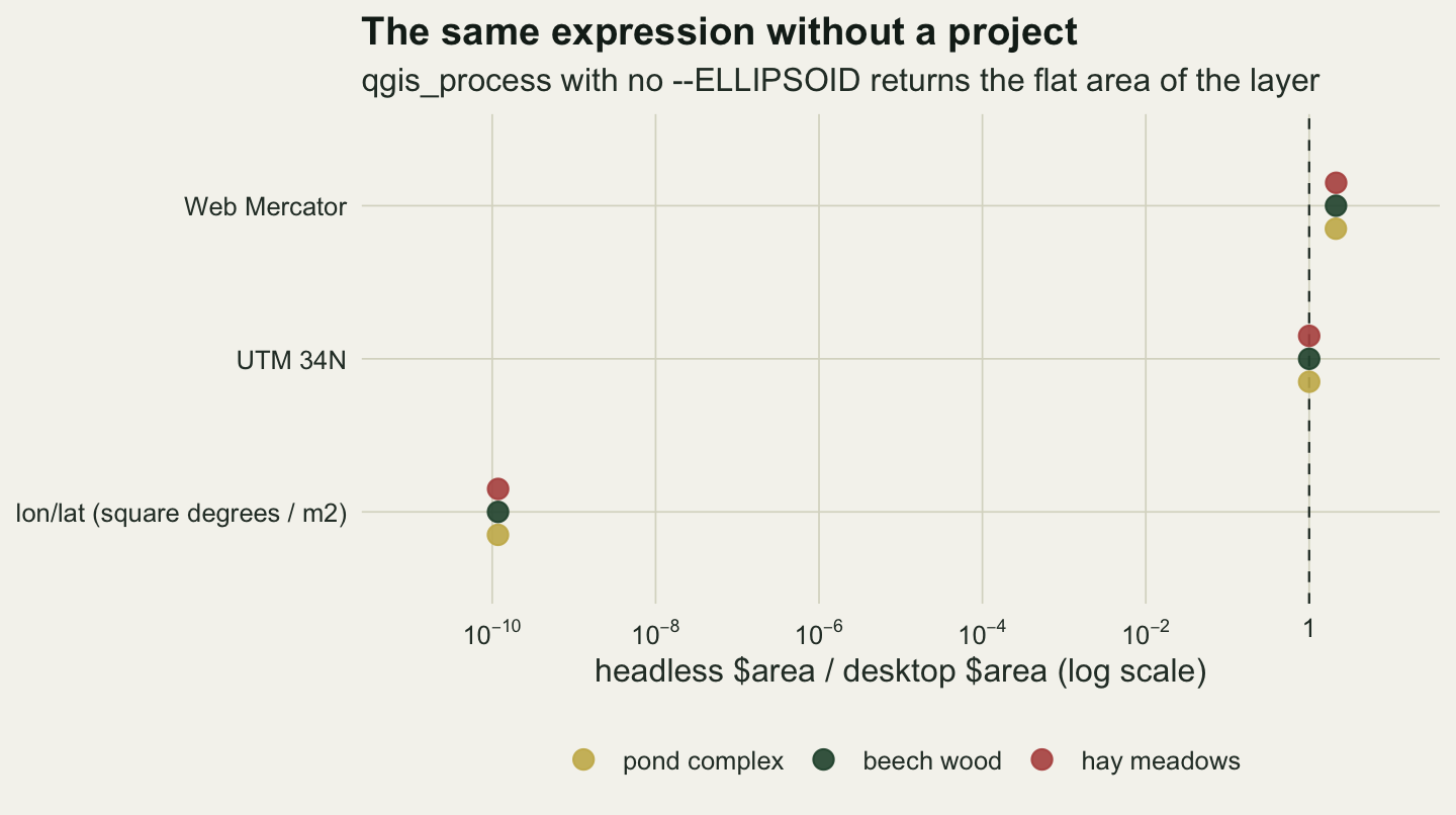
$area expression returns from qgis_process with no ellipsoid, as a multiple of what it returns in a desktop project that took its CRS from the layer. On the lon/lat layer the headless value is in square degrees. Logarithmic axis.
The trap is not limited to the field calculator. Vector > Geometry Tools > Add geometry attributes has a Calculate using option whose third choice is Ellipsoidal, and it reads the ellipsoid from the same place.
qgis_process run qgis:exportaddgeometrycolumns -- INPUT=patches-4326.gpkg CALC_METHOD=2 OUTPUT=qgis-addgeom-none.csv
qgis_process run qgis:exportaddgeometrycolumns --ELLIPSOID=EPSG:7030 -- INPUT=patches-4326.gpkg CALC_METHOD=2 OUTPUT=qgis-addgeom-wgs84.csv
ag_none <- read.csv("qgis-addgeom-none.csv"); ag_wgs <- read.csv("qgis-addgeom-wgs84.csv")
ag_flat <- max(abs(ag_none$area - q_ll$planar)); ag_ell <- max(abs(ag_wgs$area - a_ell))
gap_perim <- max(abs(ag_wgs$perimeter - perim_r))Asked for Ellipsoidal with no ellipsoid, it wrote square degrees, the same values as area($geometry), with a largest difference of 0. Given --ELLIPSOID=EPSG:7030, it wrote the ellipsoidal area, 25.808 square millimetres from st_geod_area(). Its perimeter column follows the same rule as the area: with the ellipsoid set it matches st_geod_length() on the patch outlines to within floating-point rounding. The help text of $perimeter in the field calculator describes the same rule, ellipsoidal with an ellipsoid and planimetric without one. In a script, give every call that measures an ellipsoid explicitly, or point it at the project you would have used in the desktop.
How close each pair came
sq_mm <- function(v) sprintf("%.3f square mm", 1e6 * v)
corr <- data.frame(
  qgis = c("`$area`, project ellipsoid WGS 84, square metres",
           "`$area`, project ellipsoid WGS 84, hectares",
           "`$area`, project ellipsoid Krassowsky 1940",
           "`$area`, custom sphere 6371010 m, lon/lat layer only (3.34)",
           "`area($geometry)`, UTM layer", "`area($geometry)`, Web Mercator layer",
           "`area($geometry)`, lon/lat layer",
           "`$area`, *None / Planimetric*, lon/lat layer",
           "`$area` in `qgis_process`, no ellipsoid"),
  r = c("`st_geod_area(x)`, or `st_area(x)` with `sf_use_s2(FALSE)`",
        "`st_geod_area(x) / 1e4`",
        "`st_geod_area(x)` with the Krassowsky ellipsoid attached",
        "`st_area(x)`, the default", "`st_area(x_utm)`", "`st_area(x_mercator)`",
        "`st_area(st_set_crs(x, NA))`",
        "`st_area(st_set_crs(x, NA)) * 12392029030.5`",
        "the same as `area($geometry)`"),
  gap = c(sq_mm(gap_ell), sq_mm(gap_ha * 1e4), sq_mm(gap_kr), sq_mm(gap_s2), sq_mm(gap_utm),
          sq_mm(gap_merc), "floating-point rounding (square degrees)",
          sq_mm(gap_plan), sprintf("%g (identical columns)", flat_gap)))
knitr::kable(corr, col.names = c("QGIS", "R partner", "largest gap"),
caption = "Each QGIS area and the R call that reproduces it, largest gap over the three patches.")| QGIS | R partner | largest gap |
|---|---|---|
$area, project ellipsoid WGS 84, square metres |
st_geod_area(x), or st_area(x) with sf_use_s2(FALSE) |
25.808 square mm |
$area, project ellipsoid WGS 84, hectares |
st_geod_area(x) / 1e4 |
25.808 square mm |
$area, project ellipsoid Krassowsky 1940 |
st_geod_area(x) with the Krassowsky ellipsoid attached |
58.741 square mm |
$area, custom sphere 6371010 m, lon/lat layer only (3.34) |
st_area(x), the default |
1.334 square mm |
area($geometry), UTM layer |
st_area(x_utm) |
2.973 square mm |
area($geometry), Web Mercator layer |
st_area(x_mercator) |
5.472 square mm |
area($geometry), lon/lat layer |
st_area(st_set_crs(x, NA)) |
floating-point rounding (square degrees) |
$area, None / Planimetric, lon/lat layer |
st_area(st_set_crs(x, NA)) * 12392029030.5 |
1.669 square mm |
$area in qgis_process, no ellipsoid |
the same as area($geometry) |
0 (identical columns) |
In that table x is the longitude and latitude layer and st_geod_area comes from lwgeom. The hectares row is compared after converting the gap back to square metres.
dev_levels <- c("Krassowsky ellipsoid", "sphere, sf default", "UTM 34N, flat",
                "lon/lat, None / Planimetric", "Web Mercator, flat")
dev_df <- data.frame(
  patch  = factor(rep(patches$patch, 5), levels = patches$patch),
  method = factor(rep(dev_levels, each = 3), levels = dev_levels),
  pct = c(kr_pct, sph_pct, utm_pct, plan_pct, merc_pct))
dev_df$panel <- factor(ifelse(dev_df$method %in% dev_levels[4:5], "far off", "close answers"),
                       levels = c("close answers", "far off"))
ggplot(dev_df, aes(pct, method, colour = patch)) +
  geom_vline(xintercept = 0, colour = te_body, linewidth = 0.4) +
  geom_point(size = 3, alpha = 0.9, position = position_dodge(width = 0.45)) +
  facet_wrap(~ panel, scales = "free") +
  scale_x_continuous(breaks = function(lims) pretty(lims, 4),
                     expand = expansion(mult = c(0.08, 0.12))) +
  scale_colour_manual(values = c(te_gold, te_forest, te_rust), name = NULL) +
  labs(x = "difference from WGS 84 ellipsoid (per cent)", y = NULL,
       title = "Other answers, against the WGS 84 ellipsoid",
       subtitle = "note the two horizontal scales") +
  theme_datasheet() + theme(legend.position = "bottom")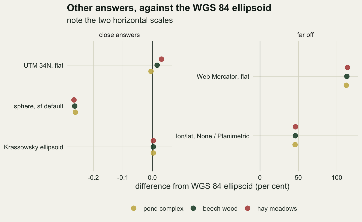
The two far ones are the settings to avoid for area on these layers: a flat area in Web Mercator, and None / Planimetric on a longitude and latitude layer.
What to report
Say which area you computed and on what surface, because “area was calculated in QGIS” names several different numbers. The usual choice for habitat patches is the ellipsoidal area on WGS 84: in QGIS, $area with Project > Properties > General, Measurements frame, showing WGS 84 as the ellipsoid, and in R st_area() with sf_use_s2(FALSE), or lwgeom::st_geod_area(), on the layer in longitude and latitude. Those two are the same computation and can be cited as one. Give the unit as well; if the project’s Units for area measurements is hectares, the QGIS column is st_geod_area(x) / 1e4. If you used the sf default, say it was measured on a sphere; the gap is 0.26 per cent at this latitude. If you used a flat area in a projected CRS, name the CRS, because the answer depends on it. If a QGIS step ran through qgis_process or a script, give the --ELLIPSOID or --PROJECT_PATH it ran with, and check one feature against the desktop before trusting the column.
Where this comes from in the QGIS source
The R side of this page ran on sf 1.1.1 (Pebesma 2018) and lwgeom 0.2.17, over PROJ 9.5.1 and GEOS 3.13.0. The QGIS files were produced by QGIS 3.34.4 on Linux, over PROJ 9.4.0. The explanations above were checked in the QGIS source, in the 3.34, 3.40 and 3.44 branches and on master, on 2026-09-25. The QGIS measuring class, QgsDistanceArea in src/core/qgsdistancearea.cpp, computes a polygon area with geod_polygon_compute() from PROJ’s geodesic.h, the C version of Karney’s algorithms; the copy of liblwgeom inside lwgeom calls the same function in ptarray_area_spheroid() when built against PROJ 4.9 or later. The QGIS side of that is the same in all four branches. The first layer sets the project ellipsoid in src/gui/layertree/qgslayertreemapcanvasbridge.cpp, through QgsProject::setCrs(crs, adjustEllipsoid) with adjustEllipsoid true unless planimetric measurement is set, and measure\planimetric=false ships in resources/qgis_global_settings.ini. The desktop field calculator (src/gui/vector/qgsfieldcalculator.cpp) passes the project’s ellipsoid and area unit to the expression, and the factor of 12392029030.5 square metres per square degree is DEG2_TO_M2 in src/core/qgsunittypes.cpp. Headless, src/process/qgsprocess.cpp leaves the ellipsoid empty unless --ELLIPSOID is given, and src/analysis/processing/qgsalgorithmfieldcalculator.cpp passes that empty name and an unknown area unit on, so the distance calculator stays at None and nothing is converted. For the custom sphere, src/core/proj/qgsellipsoidutils.cpp in 3.34 gives a PARAMETER: ellipsoid no longitude and latitude system; from 3.40 it builds one, and QgsDistanceArea::setFromParams() hands it to the coordinate transform.
Honest limits
The exact agreements rest on shared code, and that cuts both ways. QGIS and lwgeom agree to square millimetres because both call Karney’s routine inside PROJ; the R numbers on this page are recomputed wherever it is built, while the QGIS numbers were computed once, in a container running PROJ 9.4.0, and read back from files. A different PROJ underneath either side can move the last digits, and a copy of liblwgeom built without PROJ’s geodesic code falls back to an older series approximation, which was not tested. The Krassowsky case reproduces what QGIS does, which is to measure WGS 84 coordinates on another ellipsoid without a datum shift. That is a convention, the datum shift in R used whichever Pulkovo transformation PROJ picked on the build machine, and both effects are a few thousandths of a per cent or less on patches of this size.
The patches are three smooth outlines of 0.80 to 12.74 square kilometres at one latitude, with edges a few hundred metres long. QGIS and lwgeom treat each edge as a geodesic, s2 as a great circle and a flat area as a straight line in the projection. For short edges those are the same line; for a boundary of a few long straight segments, such as a grid cell tens of kilometres wide, they are not, and that difference was not measured here. The desktop behaviour was established from the source code and from PyQGIS making the same call the desktop makes, and the project settings were tested by passing saved projects to qgis_process, not by clicking through the dialogs; it holds for the shipped defaults, and an organisation can ship a different qgis_global_settings.ini. The custom sphere failing on projected layers was seen on 3.34; the 3.40 and later source contains the fix but was not run.
References
Karney CFF 2013 Journal of Geodesy 87(1):43-55 (10.1007/s00190-012-0578-z)
Pebesma E 2018 The R Journal 10(1):439-446 (10.32614/RJ-2018-009)
Pebesma E, Bivand R 2023 Spatial Data Science: With Applications in R (ISBN 9780429459016)