---
title: "Slope and aspect: what a DEM does not measure"
description: "Slope depends on the neighbourhood rule through roughness and on cell size through roughness and landform, and aspect is an angle to split into two components."
date: "2026-08-12 12:00"
date-modified: "2026-10-14"
categories: [R, terra, spatial, raster data, ecology tutorial]
image: thumbnail.png
image-alt: "Two scatter panels of plot richness, one against aspect in degrees forming a U shape crossed by a gently falling straight line, and one against northness rising along a steep straight line."
---
*Corrected 14 October 2026: the roughness section said the neighbourhood gap is roughness and nothing else and that steepness plays no part in it; it now says the gap needs roughness and that its size for a given roughness also depends on how steep the ground is. The closing limits said a noisy water surface does the same damage to a mean as a flat one; they now say it still puts meaningless bearings into the analysis but does not pull a circular mean the way a block of one bearing does.*
*Corrected 7 October 2026: the description said slope depends on both the neighbourhood rule and the cell size through surface roughness; it now says the cell size also works through the landform, as the body shows. The closing limits called independent noise the optimistic case for all the effects above; they now say correlated error of the same size shrinks the neighbourhood gap but survives coarsening better, so the flat coarse-grid columns are the optimistic case.*
*Corrected 30 September 2026: the flat-ground section said every cell of a flat lake comes back with the same easterly aspect; it now reports the first cell only and explains that the bearing on flat ground depends on floating-point residue and on the terra version.*
An elevation model measures elevation. Slope, aspect, roughness and every other terrain variable are things you compute from it, and each one carries decisions: which neighbouring cells go into the estimate, how large those cells are, and what the resulting number is allowed to mean once it reaches a model.
None of those decisions produce an error. They produce a different covariate, and the model fits either one.
## A DEM with the roughness a real one has
Real elevation models are not smooth. A photogrammetric or radar product carries a metre or two of vertical noise at the cell scale, and that noise is the hinge of everything below, so it goes in from the start rather than being added as an afterthought.
```{r setup}
#| message: false
#| warning: false
library(terra)
library(ggplot2)

te_paper  <- "#f5f4ee"
te_ink    <- "#16241d"
te_body   <- "#2c3a31"
te_forest <- "#275139"
te_rust   <- "#b5534e"
te_gold   <- "#c9b458"
te_line   <- "#dad9ca"

theme_datasheet <- function() {
  theme_minimal(base_size = 12) +
    theme(plot.background  = element_rect(fill = te_paper, colour = NA),
          panel.background = element_rect(fill = te_paper, colour = NA),
          panel.grid.major = element_line(colour = te_line, linewidth = 0.3),
          panel.grid.minor = element_blank(),
          text             = element_text(colour = te_body),
          plot.title       = element_text(colour = te_ink, face = "bold"),
          axis.text        = element_text(colour = te_body))
}

make_dem <- function(noise) {
  r <- rast(xmin = 400000, xmax = 410000, ymin = 5050000, ymax = 5060000,
            resolution = 25, crs = "EPSG:32634")
  xy <- xyFromCell(r, 1:ncell(r))
  xs <- (xy[, 1] - 400000) / 1000
  ys <- (xy[, 2] - 5050000) / 1000
  values(r) <- 500 + 60 * sin(xs * 2.2) + 75 * cos(ys * 1.7) +
    45 * sin((xs + ys) * 1.3) +
    120 * exp(-(((xs - 3.2)^2 + (ys - 6.4)^2) / 3)) +
    rnorm(ncell(r), 0, noise)
  names(r) <- "elevation"
  r
}

set.seed(20260812)
dem <- make_dem(noise = 1.5)
dem
```
Four hundred rows of 25 metre cells over a ten kilometre block, with about `r sprintf("%.0f", diff(range(values(dem))))` metres of relief. The terrain underneath is smooth; the 1.5 metres of noise is the part a real product would carry.
## Which neighbours count
`terrain` offers two neighbourhood rules. With `neighbors = 8` it takes a distance-weighted finite difference over all eight cells around the focal one, which is the Horn method most GIS software uses by default. With `neighbors = 4` it uses only the cells sharing an edge. Both are defensible; they do not return the same number.
```{r neighbours}
slope8 <- terrain(dem, v = "slope", unit = "degrees", neighbors = 8)
slope4 <- terrain(dem, v = "slope", unit = "degrees", neighbors = 4)

global(c(slope8, slope4), c("mean", "max"), na.rm = TRUE)
```
```{r gap}
gap <- values(slope4)[, 1] - values(slope8)[, 1]
round(c(mean_of_map      = mean(gap, na.rm = TRUE),
        median_abs_cell  = median(abs(gap), na.rm = TRUE),
        p90_abs_cell     = quantile(abs(gap), 0.9, na.rm = TRUE),
        max_abs_cell     = max(abs(gap), na.rm = TRUE)), 3)
```
Averaged over the map the two rules differ by `r sprintf("%.2f", mean(gap, na.rm = TRUE))` degrees, which sounds like nothing. Cell by cell the typical disagreement is `r sprintf("%.2f", median(abs(gap), na.rm = TRUE))` degrees, a tenth of the map goes over `r sprintf("%.1f", quantile(abs(gap), 0.9, na.rm = TRUE))`, and the worst cell differs by `r sprintf("%.1f", max(abs(gap), na.rm = TRUE))`. A study that extracts slope at plot locations gets the cell-level number, not the map-level one.
## Which cell size
The other decision is the grain. Coarsening the DEM and recomputing is not the same as computing on the fine grid and averaging, because slope is not a linear function of elevation.
```{r grain}
grain_row <- function(f) {
  r <- if (f == 1) dem else aggregate(dem, fact = f, fun = "mean")
  s <- terrain(r, v = "slope", unit = "degrees")
  data.frame(cell_m = f * 25,
             mean = global(s, "mean", na.rm = TRUE)[1, 1],
             p95  = global(s, function(v, ...) quantile(v, 0.95, na.rm = TRUE))[1, 1],
             max  = global(s, "max", na.rm = TRUE)[1, 1])
}
grain <- do.call(rbind, lapply(c(1, 2, 4, 8, 16), grain_row))
round(grain, 2)
```
The mean loses about a degree over that range and the steepest cell loses five: `r sprintf("%.1f", grain$max[1])` degrees at 25 metres against `r sprintf("%.1f", grain$max[nrow(grain)])` at 400 metres. A species that responds to steep ground has a covariate whose top end depends on the product you downloaded.
## Roughness drives one of those, and only part of the other
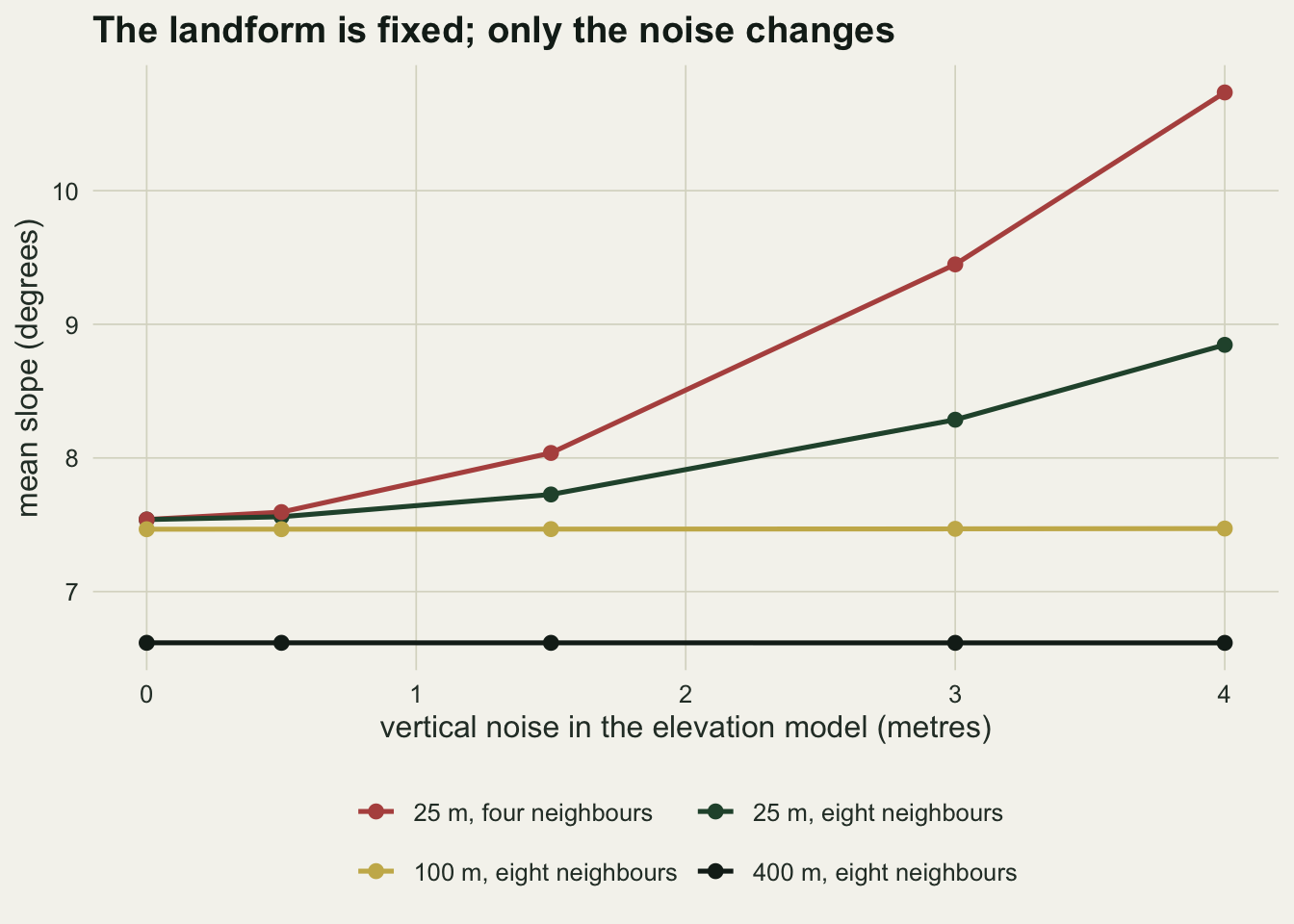
It is tempting to fold the two sections above into one problem. Rebuild the DEM at several noise levels, holding the underlying landform fixed, and the table says how much of that is right.
```{r roughness}
sweep_noise <- function(nz) {
  set.seed(20260812)
  r  <- make_dem(nz)
  s8 <- terrain(r, v = "slope", unit = "degrees", neighbors = 8)
  s4 <- terrain(r, v = "slope", unit = "degrees", neighbors = 4)
  s1 <- terrain(aggregate(r, fact = 4, fun = "mean"), v = "slope",
                unit = "degrees")
  s2 <- terrain(aggregate(r, fact = 16, fun = "mean"), v = "slope",
                unit = "degrees")
  data.frame(noise_m = nz,
             n8_25m  = global(s8, "mean", na.rm = TRUE)[1, 1],
             n4_25m  = global(s4, "mean", na.rm = TRUE)[1, 1],
             n8_100m = global(s1, "mean", na.rm = TRUE)[1, 1],
             n8_400m = global(s2, "mean", na.rm = TRUE)[1, 1])
}
rough <- do.call(rbind, lapply(c(0, 0.5, 1.5, 3, 4), sweep_noise))
round(rough, 3)
```
The neighbourhood gap needs roughness. On a noiseless surface the two rules give the same mean slope to three decimal places; at four metres of noise they are `r sprintf("%.2f", rough$n4_25m[nrow(rough)] - rough$n8_25m[nrow(rough)])` degrees apart, and the eight-neighbour estimate on the fine grid has risen by `r sprintf("%.1f", rough$n8_25m[nrow(rough)] - rough$n8_25m[1])` degrees over a landform that never changed.
The grain is two effects at once, and the two coarse columns separate them. Read down either coarse column and it barely moves: coarsening removes the noise-driven inflation, so the 100 metre and 400 metre estimates are almost the same at every noise level. Read across the noiseless top row and they are not equal to the fine-grid value: 400 metre cells give `r sprintf("%.2f", rough$n8_400m[1])` degrees against `r sprintf("%.2f", rough$n8_25m[1])` at 25 metres, a loss of `r sprintf("%.2f", rough$n8_25m[1] - rough$n8_400m[1])` degrees with no noise in the model at all. That part is the landform being averaged away, and no amount of cleaning the elevation data will bring it back.
```{r fig-roughness}
#| fig-cap: "Mean slope over the same landform at five levels of vertical noise, for two neighbourhood rules at 25 metres and for the same DEM aggregated to 100 and to 400 metres."
#| fig-alt: "Line chart with vertical noise in metres on the x axis and mean slope on the y axis. Two lines starting together near seven and a half degrees rise and separate as noise increases, the four-neighbour line rising faster. A third line for the 100 metre grid runs flat just below where they started, and a fourth for the 400 metre grid runs flat about a degree lower again."
long <- data.frame(
  noise = rep(rough$noise_m, 4),
  slope = c(rough$n8_25m, rough$n4_25m, rough$n8_100m, rough$n8_400m),
  rule  = rep(c("25 m, eight neighbours", "25 m, four neighbours",
                "100 m, eight neighbours", "400 m, eight neighbours"),
              each = nrow(rough)))
long$rule <- factor(long$rule, levels = c("25 m, four neighbours",
                                          "25 m, eight neighbours",
                                          "100 m, eight neighbours",
                                          "400 m, eight neighbours"))

ggplot(long, aes(x = noise, y = slope, colour = rule)) +
  geom_line(linewidth = 0.9) +
  geom_point(size = 2.2) +
  scale_colour_manual(values = c(te_rust, te_forest, te_gold, te_ink)) +
  labs(x = "vertical noise in the elevation model (metres)",
       y = "mean slope (degrees)",
       colour = NULL,
       title = "The landform is fixed; only the noise changes") +
  guides(colour = guide_legend(nrow = 2, byrow = TRUE)) +
  theme_datasheet() +
  theme(legend.position = "bottom")
```
That is the rule worth carrying away, in two halves. Whether the neighbourhood rule matters at all is set by how rough the surface is at the cell scale: on a smooth surface the two rules agree. How far apart roughness pushes them also depends on how steep the ground is, because the same noise inflates a gentle gradient more than a steep one. Whether the cell size matters is set by both: by the roughness, which coarsening removes, and by the shape of the landform itself, which coarsening also removes. It is why a one metre LiDAR model and a thirty metre radar model of the same hillside disagree about slope in a way that no reprojection fixes, and why the disagreement does not go away when the elevation data are clean.
## Aspect is an angle
Slope is a magnitude and behaves like one. Aspect is a compass bearing, and the moment it enters an ordinary summary or an ordinary model it stops behaving.
```{r aspect}
asp <- terrain(dem, v = "aspect", unit = "degrees")
a   <- values(asp)[, 1]
ar  <- a * pi / 180

c(arithmetic_mean = mean(a, na.rm = TRUE),
  circular_mean   = (atan2(mean(sin(ar), na.rm = TRUE),
                           mean(cos(ar), na.rm = TRUE)) %% (2 * pi)) * 180 / pi)
```
The arithmetic mean puts the average bearing at `r sprintf("%.0f", mean(a, na.rm = TRUE))` degrees, which is all but due south. The circular mean puts it at `r sprintf("%.0f", (atan2(mean(sin(ar), na.rm = TRUE), mean(cos(ar), na.rm = TRUE)) %% (2 * pi)) * 180 / pi)` degree, which is all but due north. Averaging bearings as if they were numbers pulls the answer towards the middle of the 0 to 360 range, and the pull is as strong as the amount of mass sitting either side of the cut at north: those values are treated as far apart on the scale when they are neighbours on the circle. Aspect over a whole landscape always has mass either side, so the pull is always there. It shows here as an apparent reversal only because the circular mean happens to be near north; a landscape whose bearings clustered around south would give an arithmetic mean close to right, by accident.
There is a second trap on flat ground, where aspect is undefined and something has to be returned anyway.
```{r flat}
lake <- dem
flat_cells <- cellFromRowColCombine(lake, 100:160, 100:160)
values(lake)[flat_cells] <- 470

asp_lake   <- terrain(lake, v = "aspect", unit = "degrees")
slope_lake <- terrain(lake, v = "slope",  unit = "degrees")
inner      <- cellFromRowColCombine(lake, 105:155, 105:155)

values(asp_lake)[inner[1]]
c(every_flat_cell_the_same = all(values(asp_lake)[inner] == 90),
  slope_exactly_zero       = values(slope_lake)[inner[1]] == 0)
```
The first cell of the lake comes back as `r sprintf("%.0f", values(asp_lake)[inner[1]])` degrees, roughly east, although the ground there is flat. The bearing returned on flat ground is set by floating-point residue in the gradient and by the terra version, not by the terrain: the first line of the check asks whether every cell is exactly 90, which some versions return and others do not. Put a floodplain, a reservoir or a filled sink into an aspect analysis and it arrives as a block of cells with an arbitrary bearing and no missing values to warn you. The slope on those cells is not exactly zero either, because the gradient runs through floating point, which is why the second line reads `FALSE`: the test for flat ground is a small tolerance, not equality with zero.
## Splitting the bearing
The fix is the same one used for any circular predictor. Split the angle into its two components, northness and eastness, and let the model have both.
```{r northness}
northness <- cos(ar)
eastness  <- sin(ar)

set.seed(11)
idx <- sample(which(!is.na(northness)), 300)
plots <- data.frame(elev   = values(dem)[idx, 1],
                    aspect = a[idx],
                    north  = northness[idx],
                    east   = eastness[idx])

# richness really does depend on aspect, through northness alone
plots$rich <- 18 + 4 * plots$north - 0.02 * (plots$elev - 500) +
              rnorm(nrow(plots), 0, 2.2)
```
```{r models}
m_degrees <- lm(rich ~ aspect + elev, data = plots)
m_split   <- lm(rich ~ north + east + elev, data = plots)

round(coef(summary(m_degrees)), 4)
round(coef(summary(m_split)), 4)
c(r2_degrees = summary(m_degrees)$r.squared,
  r2_split   = summary(m_split)$r.squared)
```
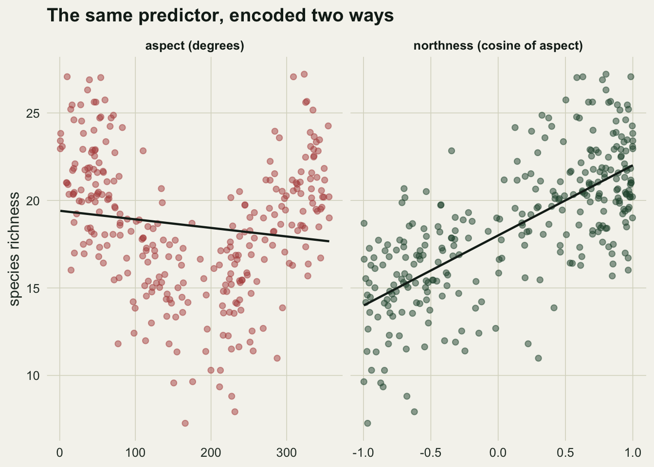
The model with aspect in degrees returns a coefficient of `r sprintf("%.4f", coef(m_degrees)[["aspect"]])` per degree with a p value of `r sprintf("%.3f", coef(summary(m_degrees))["aspect", 4])`. It is significant at the conventional threshold and it is meaningless: it asserts that richness declines steadily as the bearing runs from 0 to 359 and then jumps back up at the wrap. The figure below shows what the data actually do, and what the straight line does instead of following it. The degrees model's R squared of `r sprintf("%.2f", summary(m_degrees)$r.squared)` against the split model's `r sprintf("%.2f", summary(m_split)$r.squared)` is the cost.
The split model is also readable. The two coefficients are the components of a single vector, so their length is the amplitude of the aspect effect and their direction is the bearing the response prefers.
```{r amplitude}
b <- coef(m_split)
c(amplitude       = sqrt(b[["north"]]^2 + b[["east"]]^2),
  preferred_deg   = (atan2(b[["east"]], b[["north"]]) %% (2 * pi)) * 180 / pi)
```
The simulation put an amplitude of 4 on due north; the fit recovers `r sprintf("%.2f", sqrt(b[["north"]]^2 + b[["east"]]^2))` pointing `r sprintf("%.0f", (atan2(b[["east"]], b[["north"]]) %% (2 * pi)) * 180 / pi)` degrees east of north. The eastness coefficient on its own does not clear the conventional threshold, which is the right answer: the simulation prefers north emphatically and prefers east over west not at all.
```{r fig-aspect}
#| fig-cap: "Plot richness against aspect in degrees and against northness, from the same 300 plots."
#| fig-alt: "Two scatter panels of 300 points. In the left panel richness against aspect in degrees is high at both ends and low in the middle, a U shape with a gently falling straight line drawn across it. In the right panel richness against northness rises from low on the left to high on the right along a steep straight line that follows the points."
sc <- rbind(
  data.frame(x = plots$aspect, y = plots$rich, panel = "aspect (degrees)"),
  data.frame(x = plots$north,  y = plots$rich, panel = "northness (cosine of aspect)"))
sc$panel <- factor(sc$panel, levels = unique(sc$panel))

ggplot(sc, aes(x = x, y = y)) +
  geom_point(aes(colour = panel), alpha = 0.5, size = 1.8) +
  geom_smooth(method = "lm", formula = y ~ x, se = FALSE,
              colour = te_ink, linewidth = 0.8) +
  facet_wrap(~ panel, scales = "free_x") +
  scale_colour_manual(values = c(te_rust, te_forest)) +
  labs(x = NULL, y = "species richness",
       title = "The same predictor, encoded two ways") +
  theme_datasheet() +
  theme(legend.position = "none",
        strip.text = element_text(colour = te_ink, face = "bold"))
```
## What to record
Three lines in the methods cover all of it: the cell size of the elevation model and where it came from, the neighbourhood rule used for slope, and the encoding used for aspect. None of them is a judgement call anyone will argue with, and leaving them out makes the analysis unrepeatable in a way that is invisible.
If two products are available, computing on the finer one and aggregating the derived variable is usually closer to what the organism experiences than computing on the coarse one, but that is a claim about the organism and it should be argued rather than assumed. What is not optional is picking one and saying so.
## Honest limits
The noise in the DEM here is independent between cells, and real elevation error is not: it is spatially correlated, which makes it look more like terrain and less like noise. For a given error magnitude that shrinks the neighbourhood gap, which feeds on differences between adjacent cells, but it also lets more of the error survive coarsening, so the flat coarse-grid columns above are the optimistic case.
`terrain` implements a small number of the published slope algorithms. Others exist, including least-squares plane fits and second-order finite differences over larger windows, and the differences between them are of the same order as the ones measured here. Nothing above says the eight neighbour rule is right; it says the two are not interchangeable.
The lake demonstration uses a perfectly flat block, which is a strong version of the problem. A real water surface in a DEM usually carries a little noise, and then the aspect is not one near-constant bearing but a uniform scatter over the whole compass, which is harder to spot and still puts bearings that mean nothing into the analysis, although with no preferred direction it does not pull a circular mean the way a block of one bearing does.
Northness and eastness here are the plain cosine and sine of the bearing, which treats a north-facing cell on a one degree slope as the equal of a north-facing cell on a thirty degree one. Where slope varies widely, weighting them by the slope is the better covariate, and on a DEM that contains water or floodplain it also disposes of the block of spurious east-facing cells above. This DEM has almost no flat ground, so nothing here depends on it.
The richness model is a straight line in northness because the simulation put one there. A real response to aspect can be asymmetric, with a sharper penalty on the sun-facing side than the shaded side gains, and the two component split cannot represent that; it fits one cycle and one amplitude. Where the asymmetry matters, a smooth term on the two components together is the next step rather than a second harmonic on the raw bearing.
## References
Horn BKP 1981 Proceedings of the IEEE 69(1):14-47 (10.1109/PROC.1981.11918)
Zevenbergen LW, Thorne CR 1987 Earth Surface Processes and Landforms 12(1):47-56 (10.1002/esp.3290120107)
Hijmans RJ 2020 terra: Spatial Data Analysis, R package (10.32614/CRAN.package.terra)
## Related tutorials
- [Raster basics with terra](../terra-raster-basics/)
- [LiDAR height normalisation on slopes](../lidar-height-normalisation-on-slopes/)
- [Checking a remote sensing covariate](../checking-a-remote-sensing-covariate/)
- [Reprojecting a raster in QGIS and R: opposite defaults](../reprojecting-a-raster-in-qgis-and-r/)