LiDAR height normalisation on slopes

Normalising a LiDAR point cloud with a cell minimum invents metres of canopy on a slope. A simulation measures the bias and what it does to an ecological model.

A forest structure study in a mountain catchment: sixty square kilometres of mixed conifer between seven hundred and nineteen hundred metres, an airborne laser survey flown at four pulses per square metre, and three hundred point count stations where a canopy-nesting passerine was surveyed through one breeding season. The habitat covariate is canopy height. It is not measured in the field and it is not, strictly, downloaded either: it is computed, by taking the point cloud, subtracting a ground elevation from every return, and reducing each twenty metre cell to one number, either the tallest normalised return or the ninety-fifth percentile of them. Height percentiles from a normalised cloud are the standard predictors in laser-based forest inventory (Naesset 2002; Hyyppa et al 2008), and the same metrics moved into wildlife work because they describe vertical structure that no aerial photograph can (Vierling et al 2008).

The subtraction is where the trouble is. On flat ground almost any way of finding the ground gives the same answer, and the choice is invisible. On a slope the choices separate, and two of them separate in opposite directions. Taking the lowest return in the cell as the ground imports the cell’s own terrain drop into every height above it. Building an interpolated ground surface instead depends on ground returns, and the number of pulses that reach the forest floor collapses as the canopy closes, so the surface is held up by low vegetation exactly where the stand is tallest.

This post is the worked case of one clause in checking a remote sensing covariate. Its check 5 is that the covariate is an estimate and the model treats it as measured, and its honest limit says that a product taken from an archive “has already had somebody else’s model applied to it”. A canopy height model is that product, the somebody else’s model is the ground filter, and this post opens it and measures what comes out. The relationship to measurement error and regression dilution is a contrast rather than an extension. Classical measurement error is independent of everything, so it shrinks a slope towards zero by a factor that can be estimated and divided out. The error here is a deterministic function of the terrain. If the terrain also touches the response, and aspect, moisture and exposure mean it always does, then the covariate carries a copy of a confounder and the coefficient can move either way, including up. Dividing by a reliability ratio would make that worse.

Everything below runs on a simulated point cloud over synthetic terrain with a known true canopy height, so each estimate can be scored rather than compared with another estimate. Only ggplot2 is loaded: the cloud, the ground filter and the interpolation are a few lines of base R each, which is also the cheapest way to see what a ground filter actually does.

library(ggplot2)

te_pal <- list(forest = "#275139", green = "#2f8f63", sage = "#93a87f",
               clay = "#b5534e", gold = "#cda23f", line = "#dad9ca",
               ink = "#16241d", paper = "#f5f4ee")

theme_te <- function() {
  theme_minimal(base_size = 12) +
    theme(panel.grid.minor = element_blank(),
          panel.grid.major = element_line(colour = "#e7e6dc"),
          plot.background = element_rect(fill = "#f5f4ee", colour = NA),
          panel.background = element_rect(fill = "#f5f4ee", colour = NA),
          plot.title = element_text(face = "bold", colour = te_pal$ink),
          axis.title = element_text(colour = "#2c3a31"),
          axis.text = element_text(colour = "#2c3a31"))
}

The cloud, and what a normalisation has to do

A pulse leaving the aircraft either finds a gap and reaches the ground or is stopped by foliage. The share that reaches the ground falls with canopy closure the way transmission falls through a turbid medium, so the ground return probability is written as \(\exp(-k \cdot \text{closure})\) with \(k\) set so that an open stand returns most pulses from the floor and a closed one returns a few per cent. A pulse that is stopped returns from somewhere inside the crown: most often near the top, sometimes from a low branch or the understorey, and the height of that low return scales with the stand, because a taller stand has a taller understorey and a higher first live branch.

dens <- 4          # pulses per square metre
k_ext <- 5         # extinction coefficient for ground return probability
p_low <- 0.28      # share of canopy returns coming from the lower crown
crown_top <- 0.30  # upper returns lie within this fraction of the height below the top
low_lo <- 0.06     # lower crown returns span this fraction of the height
low_hi <- 0.45
range_sd <- 0.05   # ranging error, metres

h_above <- function(h_true, cc, n) {
  u1 <- runif(n); u2 <- runif(n); u3 <- runif(n)
  hh <- ifelse(u2 < p_low,
               h_true * (low_lo + (low_hi - low_lo) * u3),
               h_true * (1 - crown_top * (1 - (1 - u3)^(1 / 3))))
  hh[u1 < exp(-k_ext * cc)] <- 0
  hh
}

sim_tile <- function(side_m, tan_s, h_true, cc, dens_p = dens) {
  n <- round(side_m^2 * dens_p)
  xx <- runif(n, 0, side_m); yy <- runif(n, 0, side_m)
  gz <- -xx * tan_s
  hh <- h_above(h_true, cc, n)
  list(x = xx, y = yy, gz = gz, hh = hh, n = n,
       z = gz + hh + rnorm(n, 0, range_sd))
}

cell_index <- function(xx, yy, side_m, cell_m) {
  nc <- round(side_m / cell_m)
  pmin(floor(xx / cell_m), nc - 1) + pmin(floor(yy / cell_m), nc - 1) * nc
}

cc_probe <- c(0.2, 0.5, 0.8, 0.95)
print(round(rbind(closure = cc_probe,
                  ground_return_share = exp(-k_ext * cc_probe),
                  ground_returns_per_m2 = dens * exp(-k_ext * cc_probe)), 4))

                        [,1]   [,2]   [,3]   [,4]
closure               0.2000 0.5000 0.8000 0.9500
ground_return_share   0.3679 0.0821 0.0183 0.0087
ground_returns_per_m2 1.4715 0.3283 0.0733 0.0346

The terrain is a plane tilted by a chosen angle, which is the simplest surface on which the question has an answer that can be checked by hand. At 4 pulses per square metre a closure of 0.2 sends 1.472 ground returns into every square metre and a closure of 0.95 sends 0.0346, a fall of a factor of 42.5. That collapse is the second half of the post; the first half needs no canopy closure at all.

Two normalisations are compared throughout. The cell minimum takes the lowest return inside the output cell as that cell’s ground and subtracts it from the highest, which is the shortcut that needs no ground filter and no interpolation. The interpolated ground runs a crude version of what a real filter does: divide the tile into small windows, take the lowest return in each window as a ground seed, and fit a surface through the seeds. Kraus and Pfeifer (1998) built the standard version of that idea, an iterative weighted surface that pushes itself down onto the low returns; the seeds here are the first step of the same logic without the iteration.

w_m <- 5           # side of the ground filter window, metres

seed_grid <- function(d, side_m, w_m) {
  nw <- round(side_m / w_m)
  id <- cell_index(d$x, d$y, side_m, w_m)
  sz <- tapply(d$z, id, min)
  ids <- as.integer(names(sz))
  list(sx = (ids %% nw + 0.5) * w_m, sy = (ids %/% nw + 0.5) * w_m,
       sz = as.numeric(sz), ngr = as.numeric(tapply(d$hh == 0, id, sum)))
}

plane_fit <- function(sg) as.numeric(qr.solve(cbind(1, sg$sx, sg$sy), sg$sz))

One detail of that filter matters later and is easy to miss. The lowest return in a window has a position of its own, but a gridded terrain model stores one elevation per window and hangs it at the window centre. On a slope the lowest return sits at the downhill edge, so the stored elevation is too low for the place it is stored at, by roughly half the window’s own terrain drop.

A cell minimum invents canopy on a slope

Take one twenty metre cell on a twenty-five degree slope, with a stand of uniform height, and plenty of ground returns so that nothing about canopy density is in play.

h_stand <- 26
slope_demo <- 25
cell_demo <- 20
cc_open <- 0.35

set.seed(20260804)
demo <- sim_tile(cell_demo, tan(slope_demo * pi / 180), h_stand, cc_open)
z_lo <- min(demo$z)
z_hi <- max(demo$z)
chm_demo <- z_hi - z_lo
span_demo <- cell_demo * tan(slope_demo * pi / 180)

print(round(c(returns = demo$n,
              ground_returns = sum(demo$hh == 0),
              true_height = h_stand,
              cell_minimum = z_lo,
              cell_maximum = z_hi,
              chm_cell_minimum = chm_demo,
              phantom_canopy = chm_demo - h_stand,
              terrain_span = span_demo,
              half_span = span_demo / 2), 4))

         returns   ground_returns      true_height     cell_minimum 
       1600.0000         278.0000          26.0000          -9.2866 
    cell_maximum chm_cell_minimum   phantom_canopy     terrain_span 
         25.8607          35.1473           9.1473           9.3262 
       half_span 
          4.6631 

The cell holds 1600 returns of which 278 came from the ground, so the lowest return is a genuine ground return and the filter has nothing to be blamed for. The canopy height model still reports 35.15 metres for a stand that is 26 metres tall, 9.15 metres of canopy that is not there. Twenty metres of ground at twenty-five degrees falls 9.33 metres, and that is where the extra height came from: the cell minimum sits at the bottom corner of the cell and the tallest return sits near the top corner.

Figure 1: One twenty metre cell on a twenty-five degree slope, seen in cross section. Every return in the cell is projected onto the downslope axis. The lower dark line is the true ground, the upper one the true canopy top, and the two are twenty-six metres apart everywhere. The two dashed horizontal lines are the lowest and the highest return in the cell, and the distance between them is what a cell minimum normalisation reports as the canopy height.

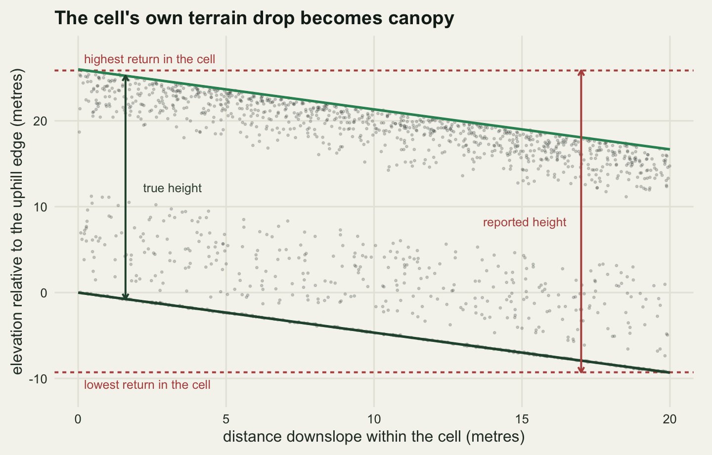
One cell is an anecdote. The sweep below runs four cell sizes across nine slope angles over a one hundred and forty metre tile, and records three quantities for each combination: the bias of the canopy height model built from the cell maximum, the bias of the ninety-fifth percentile version, and the terrain offset carried by the returns themselves, which is \(\text{ground}(x) - \min(\text{ground})\) within the cell and involves no canopy at all.

cell_grid <- c(2, 5, 10, 20)
slope_grid <- c(0, 5, 10, 15, 20, 25, 30, 35, 40)
side1 <- 140

set.seed(20260805)
res1 <- NULL
for (cm in cell_grid) {
  for (sdg in slope_grid) {
    tan_s <- tan(sdg * pi / 180)
    d <- sim_tile(side1, tan_s, h_stand, cc_open)
    id <- cell_index(d$x, d$y, side1, cm)
    zmin <- tapply(d$z, id, min)
    zmax <- tapply(d$z, id, max)
    grp <- match(id, as.integer(names(zmin)))
    hn <- d$z - zmin[grp]
    tall <- hn > 2
    p95 <- tapply(hn[tall], id[tall], quantile, probs = 0.95)
    gmin <- tapply(d$gz, id, min)
    toff <- d$gz - gmin[grp]
    res1 <- rbind(res1, data.frame(
      cell_m = cm, slope_deg = sdg,
      bias_max = mean(zmax - zmin) - h_stand,
      bias_p95 = mean(p95, na.rm = TRUE) - h_stand,
      terr_mean = mean(toff),
      terr_max = mean(tapply(toff, id, max)),
      geo_span = cm * tan_s, geo_half = cm * tan_s / 2))
  }
}
q1 <- function(cm, sdg, nm) res1[[nm]][res1$cell_m == cm & res1$slope_deg == sdg]
print(round(res1[res1$cell_m == 20, ], 3))

   cell_m slope_deg bias_max bias_p95 terr_mean terr_max geo_span geo_half
28     20         0    0.212   -0.043     0.000    0.000    0.000    0.000
29     20         5    1.738    0.975     0.874    1.748    1.750    0.875
30     20        10    3.459    2.294     1.757    3.522    3.527    1.763
31     20        15    5.254    3.818     2.677    5.352    5.359    2.679
32     20        20    7.118    5.411     3.633    7.270    7.279    3.640
33     20        25    9.107    7.097     4.653    9.314    9.326    4.663
34     20        30   11.291    9.044     5.771   11.533   11.547    5.774
35     20        35   13.728   11.222     6.979   13.989   14.004    7.002
36     20        40   16.454   13.604     8.368   16.760   16.782    8.391

print(round(res1[res1$slope_deg == 25, ], 3))

   cell_m slope_deg bias_max bias_p95 terr_mean terr_max geo_span geo_half
6       2        25   -0.322   -0.536     0.411    0.816    0.933    0.466
15      5        25    1.786    1.159     1.142    2.284    2.332    1.166
24     10        25    4.333    3.103     2.315    4.640    4.663    2.332
33     20        25    9.107    7.097     4.653    9.314    9.326    4.663

The arithmetic is exact and worth doing before reading the simulated column. A cell of side \(c\) on a slope of angle \(\theta\) spans \(c \tan\theta\) of terrain, so a return drawn at a uniformly random position inside it sits \(c\tan\theta / 2\) above the cell’s lowest ground on average, and the return nearest the uphill edge sits the full \(c\tan\theta\) above it. At twenty metres and twenty-five degrees those are 4.663 and 9.326 metres. The simulated terrain offsets are 4.653 and 9.314, which is the geometry recovered to three decimal places and confirms that nothing else is going on.

Which of the two numbers the canopy height model inherits depends on the metric. A mean return height would inherit the half span. A cell maximum inherits nearly the whole span, because the tallest return in a cell of 1600 returns is close to the uphill edge, and the measured bias at twenty metres and twenty-five degrees is 9.107 metres against a span of 9.326. The ninety-fifth percentile is not much gentler at 7.097 metres. A first guess that a twenty metre cell at twenty-five degrees buys four or five metres of phantom canopy is the half-span answer and is too kind by a factor of about 1.95: the estimator in use picks up the top of the drop, not the middle of it. Nine metres is not a decade of growth on a mixed conifer stand. It is closer to half the stand.

Figure 2: Bias of a cell minimum canopy height model against slope angle, at four cell sizes, with the canopy height held at twenty-six metres and ground returns plentiful. The dashed lines are the terrain span of each cell, the cell side times the tangent of the slope, computed with no simulation at all. The measured bias tracks the span rather than half of it, and it scales with cell size, not with the height of the stand.

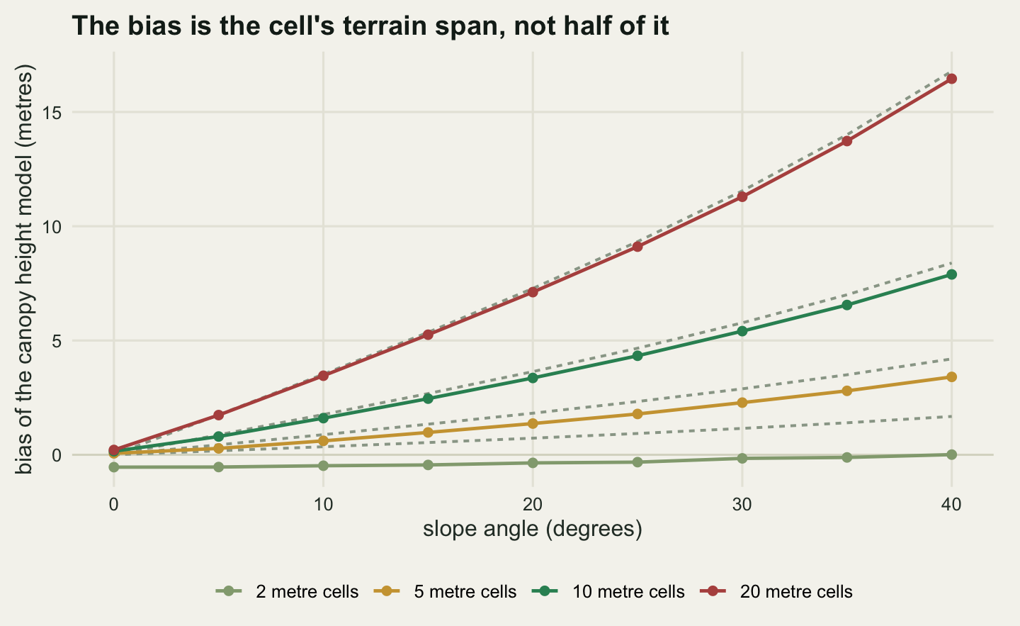
Two readings off that figure are worth keeping. The bias does not depend on the stand: it is terrain multiplied by cell size, so a short stand on a steep slope can be reported as taller than a tall stand on a flat one. And the flat-ground column is not quite zero. At two metre cells the bias at zero slope is -0.541 metres, because a cell that small holds only 16 returns and the tallest of them misses the apex of the crown. Pulse penetration into the upper canopy before a return is triggered is a real and separate downward bias, measured directly by Gaveau and Hill (2003); here it is the only thing left when the slope is taken away.

Ground returns run out under a closed canopy

The recommended alternative is to normalise against an interpolated ground surface. That surface is built from ground returns, and the supply of ground returns is not a constant of the survey. Reutebuch et al (2003) measured a lidar terrain model under a conifer canopy and found the accuracy tracking how many pulses got through; Sithole and Vosselman (2004) compared eight filter algorithms and found their errors concentrated in exactly two places, steep terrain and dense low vegetation.

The sweep below holds the terrain flat, so nothing in it is about slope, and moves canopy closure from open to nearly shut at two stand heights.

cc_grid <- c(0.20, 0.35, 0.50, 0.65, 0.80, 0.90, 0.95)
h_lev <- c(14, 26)
side2 <- 140
cell2 <- 20

set.seed(20260806)
res2 <- NULL
for (hv in h_lev) {
  for (cv in cc_grid) {
    d <- sim_tile(side2, 0, hv, cv)
    sg <- seed_grid(d, side2, w_m)
    cf <- plane_fit(sg)
    gh <- cf[1] + cf[2] * d$x + cf[3] * d$y
    hn <- d$z - gh
    id <- cell_index(d$x, d$y, side2, cell2)
    zmin <- tapply(d$z, id, min); zmax <- tapply(d$z, id, max)
    res2 <- rbind(res2, data.frame(
      h_true = hv, cc = cv,
      gr_frac = mean(d$hh == 0),
      gr_per_win = mean(sg$ngr),
      empty_win = mean(sg$ngr == 0),
      seed_lift = mean(sg$sz),
      bias_interp = mean(tapply(hn, id, max)) - hv,
      bias_cellmin = mean(zmax - zmin) - hv))
  }
}
q2 <- function(hv, cv, nm) res2[[nm]][res2$h_true == hv & res2$cc == cv]
print(round(res2[res2$h_true == 26, ], 4))

   h_true   cc gr_frac gr_per_win empty_win seed_lift bias_interp bias_cellmin
8      26 0.20  0.3681    36.8125    0.0000   -0.1060      0.1658       0.2140
9      26 0.35  0.1722    17.2156    0.0000   -0.0892      0.1615       0.2159
10     26 0.50  0.0837     8.3724    0.0000   -0.0695      0.1421       0.2035
11     26 0.65  0.0388     3.8776    0.0332    0.0239      0.0540       0.1895
12     26 0.80  0.0190     1.9031    0.1454    0.2560     -0.1772       0.1821
13     26 0.90  0.0110     1.1046    0.3253    0.6127     -0.5358       0.1634
14     26 0.95  0.0088     0.8763    0.4005    0.7557     -0.6778       0.1558

print(round(res2[res2$h_true == 14, ], 4))

  h_true   cc gr_frac gr_per_win empty_win seed_lift bias_interp bias_cellmin
1     14 0.20  0.3673    36.7296    0.0000   -0.1069      0.1869       0.2378
2     14 0.35  0.1725    17.2513    0.0000   -0.0891      0.1739       0.2268
3     14 0.50  0.0827     8.2679    0.0000   -0.0693      0.1558       0.2182
4     14 0.65  0.0389     3.8865    0.0128   -0.0320      0.1206       0.2065
5     14 0.80  0.0193     1.9298    0.1454    0.1291     -0.0405       0.1841
6     14 0.90  0.0115     1.1467    0.3189    0.3170     -0.2324       0.1725
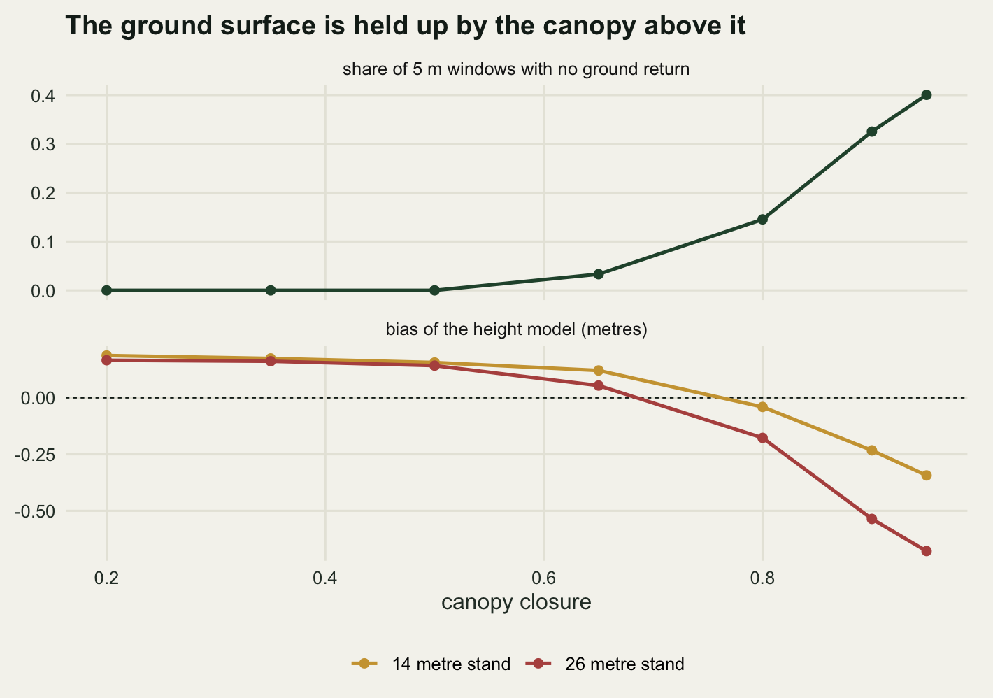
7     14 0.95  0.0080     0.8048    0.4337    0.4340     -0.3435       0.1776

At a closure of 0.2 each 5 metre window receives 36.8 ground returns and every window has some. At 0.95 the count is 0.88 and 40.1 per cent of windows have none at all. A window with no ground return still contributes a seed, because the filter has no way of knowing that the lowest return it found was a branch. In the 26 metre stand those seeds lift the ground surface by an average of 0.756 metres and the canopy height model comes back 0.678 metres short.

The lift scales with the stand, which is the part that makes this a bias rather than noise. In the 14 metre stand at the same closure the seeds lift by 0.434 metres and the shortfall is 0.343 metres. The two lifts differ by a factor of 1.74, close to the ratio of the two stand heights, 1.86. The lowest branch of a tall tree is higher off the ground than the lowest branch of a short one, so the surface is pushed up furthest under the stands whose height matters most.

The cell minimum is not the estimator that suffers here. Its bias moves from 0.214 to 0.156 metres across the whole closure range, because a twenty metre cell pools 1600 returns and at 0.95 closure that still leaves about 14 of them on the floor. Ground return sparsity is a problem for the unit the ground is estimated over, and a 5 metre filter window covers 6 per cent of the area of a twenty metre cell. That is the trade the next section is about: shrinking the ground estimation unit cuts the terrain error and raises the density error.

Figure 3: The share of five metre filter windows containing no ground return, and the resulting bias of an interpolated ground normalisation, against canopy closure on flat terrain. The lower panel carries a fourteen metre stand and a twenty-six metre stand. The bias is near zero while every window still finds the floor, and turns negative once windows start coming up empty, twice as far down in the taller stand.

The two errors meet, and only one estimator changes sign

The last two sections each held one thing fixed. Putting slope and closure on the two axes of a grid and running both estimators over it gives the net error, and the question is where the net crosses zero. The prediction to test is that a positive terrain term and a negative density term should cancel somewhere in the middle of the grid.

side3 <- 100
cell3 <- 20
cc_net <- c(0.20, 0.40, 0.60, 0.75, 0.85, 0.95)

set.seed(20260807)
res3 <- NULL
for (sdg in slope_grid) {
  tan_s <- tan(sdg * pi / 180)
  for (cv in cc_net) {
    d <- sim_tile(side3, tan_s, h_stand, cv)
    sg <- seed_grid(d, side3, w_m)
    cf <- plane_fit(sg)
    gh <- cf[1] + cf[2] * d$x + cf[3] * d$y
    hn <- d$z - gh
    id <- cell_index(d$x, d$y, side3, cell3)
    zmin <- tapply(d$z, id, min); zmax <- tapply(d$z, id, max)
    res3 <- rbind(res3, data.frame(
      slope_deg = sdg, cc = cv,
      bias_cellmin = mean(zmax - zmin) - h_stand,
      bias_interp = mean(tapply(hn, id, max)) - h_stand,
      surf_off = mean(gh - d$gz),
      empty_win = mean(sg$ngr == 0),
      half_win = w_m * tan_s / 2, span_cell = cell3 * tan_s))
  }
}
q3 <- function(sdg, cv, nm) res3[[nm]][res3$slope_deg == sdg & res3$cc == cv]
print(round(res3[res3$cc == 0.20, ], 3))

   slope_deg  cc bias_cellmin bias_interp surf_off empty_win half_win span_cell
1          0 0.2        0.211       0.170   -0.105         0    0.000     0.000
7          5 0.2        1.756       0.324   -0.249         0    0.219     1.750
13        10 0.2        3.442       0.509   -0.446         0    0.441     3.527
19        15 0.2        5.222       0.722   -0.659         0    0.670     5.359
25        20 0.2        7.135       0.952   -0.885         0    0.910     7.279
31        25 0.2        9.094       1.170   -1.113         0    1.166     9.326
37        30 0.2       11.314       1.451   -1.387         0    1.443    11.547
43        35 0.2       13.724       1.722   -1.660         0    1.751    14.004
49        40 0.2       16.486       2.051   -1.992         0    2.098    16.782

print(round(res3[res3$cc == 0.95, ], 3))

   slope_deg   cc bias_cellmin bias_interp surf_off empty_win half_win
6          0 0.95        0.151      -0.755    0.829     0.432    0.000
12         5 0.95        1.557      -0.683    0.770     0.412    0.219
18        10 0.95        3.162      -0.628    0.703     0.400    0.441
24        15 0.95        4.866      -0.588    0.659     0.418    0.670
30        20 0.95        6.648      -0.449    0.525     0.390    0.910
36        25 0.95        8.503      -0.436    0.521     0.380    1.166
42        30 0.95       10.600      -0.465    0.543     0.435    1.443
48        35 0.95       12.907      -0.309    0.384     0.422    1.751
54        40 0.95       15.312      -0.132    0.222     0.458    2.098
   span_cell
6      0.000
12     1.750
18     3.527
24     5.359
30     7.279
36     9.326
42    11.547
48    14.004
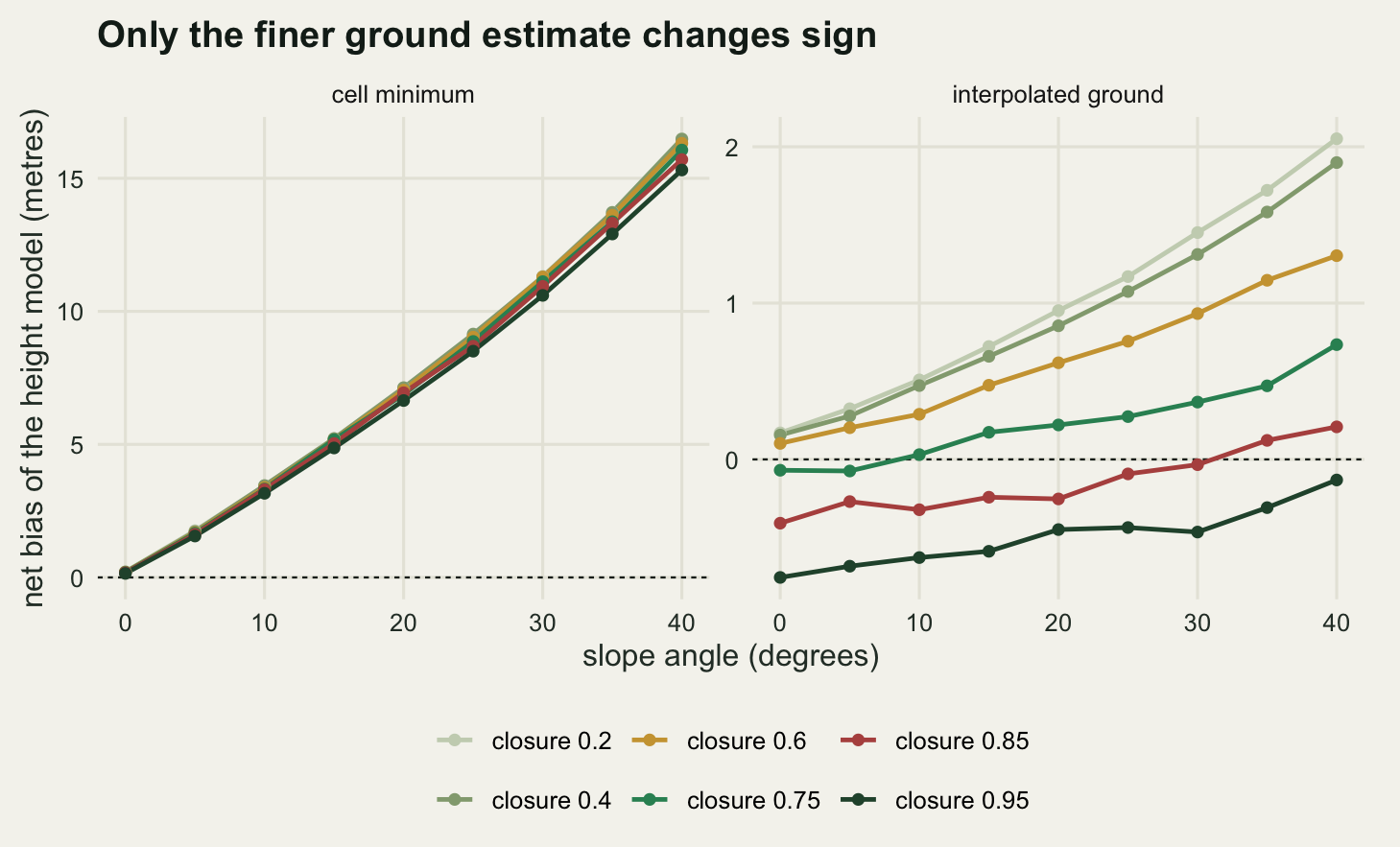
54    16.782

The open-canopy column checks the geometry of the interpolated surface. At twenty-five degrees and a closure of 0.2 the interpolated normalisation is biased by 1.17 metres against a predicted half window span of 1.166, and the fitted ground surface sits 1.113 metres below the true one. The interpolation has not removed the terrain error. It has replaced the cell’s whole terrain span with half the window’s, dividing the term by 8, and the two measured biases stand in a ratio of 7.78. The cell minimum at the same point is out by 9.094 metres.

cross_at <- function(nm) {
  vapply(cc_net, function(cv) {
    v <- res3[[nm]][res3$cc == cv]
    j <- which(v[-1] * v[-length(v)] < 0)
    if (!length(j)) return(NA_real_)
    j <- j[length(j)]
    slope_grid[j] - v[j] * (slope_grid[j + 1] - slope_grid[j]) /
      (v[j + 1] - v[j])
  }, numeric(1))
}
sign_tab <- data.frame(cc = cc_net,
                       cross_interp = cross_at("bias_interp"),
                       cross_cellmin = cross_at("bias_cellmin"))
print(round(sign_tab, 3))

    cc cross_interp cross_cellmin
1 0.20           NA            NA
2 0.40           NA            NA
3 0.60           NA            NA
4 0.75        8.540            NA
5 0.85       31.083            NA
6 0.95           NA            NA

cc_effect <- max(tapply(res3$bias_cellmin, res3$slope_deg,
                        function(v) max(v) - min(v)))
print(round(c(closure_range_on_cellmin = cc_effect,
              min_cellmin_bias = min(res3$bias_cellmin),
              max_cellmin_bias = max(res3$bias_cellmin),
              min_interp_bias = min(res3$bias_interp),
              max_interp_bias = max(res3$bias_interp),
              cells_negative_cellmin = mean(res3$bias_cellmin < 0),
              cells_negative_interp = mean(res3$bias_interp < 0)), 3))

closure_range_on_cellmin         min_cellmin_bias         max_cellmin_bias 
                   1.175                    0.151                   16.486 
         min_interp_bias          max_interp_bias   cells_negative_cellmin 
                  -0.755                    2.051                    0.000 
   cells_negative_interp 
                   0.333 

Half of the prediction came out and half did not. For the interpolated normalisation the two errors do cancel, and the slope at which they cancel climbs with closure: about 8.5 degrees at a closure of 0.75 and about 31.1 degrees at 0.85. Below the crossing the terrain term wins and the stand is reported too tall; above it the ground surface is held up and the stand is reported too short. At the two lightest closures the estimate is positive everywhere in the grid, and at 0.95 it is negative everywhere: the zero contour has left through the top of the grid, because forty degrees of slope no longer buys enough terrain error to pay for a ground surface built from 46 per cent empty windows. A catchment holding steep open ridges and closed valley bottoms sits on both sides of that contour, and the sign of its canopy height error changes across the map.

The cell minimum does not cross anywhere. Over the whole grid its bias runs from 0.151 to 16.486 metres and 0 per cent of the combinations are negative. Holding the slope fixed and sweeping closure over the whole range moves its bias by at most 1.17 metres, against a terrain span that reaches 16.78. The estimation unit is the whole twenty metre cell, and it keeps finding ground even at 0.95 closure. So the two errors are real, they do have opposite signs, and they are only comparable in size when the ground is estimated over a small enough window. The shortcut is not a case of two errors trading off. It is one error with a rounding term attached.

Figure 4: Net bias of the two normalisations over a grid of slope angle and canopy closure, at a twenty-six metre stand and twenty metre output cells. Note the very different vertical scales. The cell minimum is positive everywhere in the grid and its curves are almost stacked on one another, since closure barely moves it. The interpolated surface crosses zero, and the crossing moves to steeper ground as the canopy closes.

What a terrain-shaped error does to the model

The point of the covariate is to go into a model. Build a catchment of three hundred cells, each with its own slope angle, its own canopy closure and its own true canopy height, simulate the point cloud over each of them, and normalise both ways. True height is drawn independently of slope, which is a simplification and is deliberate: any correlation between the two would put ordinary confounding into the answer alongside the effect being measured.

n_site <- 300
side4 <- 30
core_lo <- 5
core_hi <- 25

set.seed(20260808)
slope_deg <- 45 * rbeta(n_site, 2, 3)
cc_site <- runif(n_site, 0.35, 0.95)
h_site <- pmin(pmax(rnorm(n_site, 26, 4), 12), 38)
chm_cm <- chm_in <- ngr_cell <- numeric(n_site)

for (i in seq_len(n_site)) {
  d <- sim_tile(side4, tan(slope_deg[i] * pi / 180), h_site[i], cc_site[i])
  sg <- seed_grid(d, side4, w_m)
  cf <- plane_fit(sg)
  gh <- cf[1] + cf[2] * d$x + cf[3] * d$y
  core <- d$x >= core_lo & d$x < core_hi & d$y >= core_lo & d$y < core_hi
  chm_cm[i] <- max(d$z[core]) - min(d$z[core])
  chm_in[i] <- max(d$z[core] - gh[core])
  ngr_cell[i] <- sum((d$z[core] - gh[core]) < 0.5)
}

terr <- as.numeric(scale(slope_deg))
lam_cm <- var(h_site) / var(chm_cm)
lam_in <- var(h_site) / var(chm_in)
print(round(c(mean_slope = mean(slope_deg), max_slope = max(slope_deg),
              mean_bias_cellmin = mean(chm_cm - h_site),
              sd_bias_cellmin = sd(chm_cm - h_site),
              mean_bias_interp = mean(chm_in - h_site),
              sd_bias_interp = sd(chm_in - h_site),
              cor_true_slope = cor(h_site, slope_deg),
              cor_cellmin_slope = cor(chm_cm, slope_deg),
              reliability_cellmin = lam_cm,
              reliability_interp = lam_in), 4))

         mean_slope           max_slope   mean_bias_cellmin     sd_bias_cellmin 
            18.1772             41.5534              6.4712              3.5008 
   mean_bias_interp      sd_bias_interp      cor_true_slope   cor_cellmin_slope 
             0.4128              0.4786              0.0118              0.6637 
reliability_cellmin  reliability_interp 
             0.5660              1.0298 

The catchment averages 18.2 degrees and reaches 41.6. True canopy height correlates with slope at 0.012, which is as close to nothing as a draw of 300 allows. The cell minimum covariate correlates with slope at 0.664. That single number is the whole problem: a variable built to describe vegetation has become, in large part, a map of the terrain.

The classical reading of the next step is measurement error. The reliability ratio of the cell minimum covariate is 0.566, so a textbook correction would say the coefficient comes back attenuated by that factor and can be divided back up. The response below is generated as canopy height plus a terrain effect of varying strength, with the terrain effect standing in for aspect, moisture and exposure, and the sweep asks whether the textbook reading survives.

b_true <- 0.08
sd_eps <- 0.6
g_grid <- seq(-0.8, 0.8, by = 0.2)
n_rep <- 200

set.seed(20260809)
terr_dem <- as.numeric(scale(slope_deg + rnorm(n_site, 0, 4)))
coef_tab <- NULL
for (gv in g_grid) {
  acc <- matrix(NA_real_, n_rep, 5)
  for (r in seq_len(n_rep)) {
    yv <- 2 + b_true * h_site + gv * terr + rnorm(n_site, 0, sd_eps)
    acc[r, ] <- c(coef(lm(yv ~ chm_cm))[2],
                  coef(lm(yv ~ chm_in))[2],
                  coef(lm(yv ~ h_site + terr))[2],
                  coef(lm(yv ~ chm_cm + terr))[2],
                  coef(lm(yv ~ chm_cm + terr_dem))[2])
  }
  coef_tab <- rbind(coef_tab, data.frame(
    g = gv, cellmin = mean(acc[, 1]), interp = mean(acc[, 2]),
    oracle = mean(acc[, 3]), adj_true = mean(acc[, 4]),
    adj_dem = mean(acc[, 5]),
    predicted = (b_true * cov(h_site, chm_cm) + gv * cov(terr, chm_cm)) /
      var(chm_cm)))
}
g_star <- b_true * (var(chm_cm) - cov(h_site, chm_cm)) / cov(terr, chm_cm)
print(round(coef_tab, 4))

     g cellmin interp oracle adj_true adj_dem predicted
1 -0.8 -0.0545 0.0659 0.0812   0.0812  0.0357   -0.0547
2 -0.6 -0.0304 0.0674 0.0787   0.0788  0.0422   -0.0297
3 -0.4 -0.0044 0.0728 0.0801   0.0801  0.0518   -0.0047
4 -0.2  0.0208 0.0777 0.0810   0.0810  0.0608    0.0203
5  0.0  0.0451 0.0797 0.0790   0.0790  0.0678    0.0453
6  0.2  0.0703 0.0847 0.0802   0.0803  0.0770    0.0703
7  0.4  0.0943 0.0881 0.0797   0.0798  0.0849    0.0952
8  0.6  0.1196 0.0915 0.0790   0.0791  0.0926    0.1202
9  0.8  0.1449 0.0961 0.0796   0.0797  0.1014    0.1452

print(round(c(true_coefficient = b_true,
              classical_prediction = b_true * lam_cm,
              at_zero_terrain = coef_tab$cellmin[coef_tab$g == 0],
              g_that_looks_right = g_star,
              worst_low = min(coef_tab$cellmin),
              worst_high = max(coef_tab$cellmin),
              max_pred_error = max(abs(coef_tab$predicted -
                                         coef_tab$cellmin))), 4))

    true_coefficient classical_prediction      at_zero_terrain 
              0.0800               0.0453               0.0451 
  g_that_looks_right            worst_low           worst_high 
              0.2780              -0.0545               0.1449 
      max_pred_error 
              0.0009 

With no terrain effect on the response the naive fit returns 0.0451 against a truth of 0.08, and the classical prediction for that cell is 0.0453. The textbook reading is right there and nowhere else. Turn the terrain effect on and the coefficient walks: at the strongest negative terrain effect in the sweep it is -0.0545, the wrong sign, and at the strongest positive one it is 0.1449, or 1.81 times the truth. A correctly specified fit on the true heights returns 0.0798 throughout.

The walk is not mysterious. Writing \(\hat{H}\) for the covariate and \(T\) for the terrain variable, and taking the response as \(y = a + \beta H + \gamma T + \varepsilon\), ordinary least squares on \(\hat{H}\) alone returns

\[\frac{\operatorname{Cov}(y, \hat{H})}{\operatorname{Var}(\hat{H})} = \frac{\beta \operatorname{Cov}(H, \hat{H}) + \gamma \operatorname{Cov}(T, \hat{H})}{\operatorname{Var}(\hat{H})}\]

which is a straight line in \(\gamma\). Its intercept is the classical attenuated value, and its slope is 0.1249, the regression of the covariate on the terrain. That formula reproduces the simulated coefficients to within 0.00091. It also says where the crossing is: at a terrain effect of 0.278 the biased covariate returns the true coefficient exactly, for the wrong reason, and nothing in the output distinguishes that point from a clean analysis.

Figure 5: Fitted coefficient on canopy height against the strength of a terrain effect on the response, averaged over two hundred replicates at each point. The dashed line is the true coefficient. A covariate normalised by cell minimum returns anything from the wrong sign to nearly double the truth as the terrain effect varies; the interpolated version moves much less; a fit on the true heights is flat. Classical attenuation predicts only the point where the terrain effect is zero.

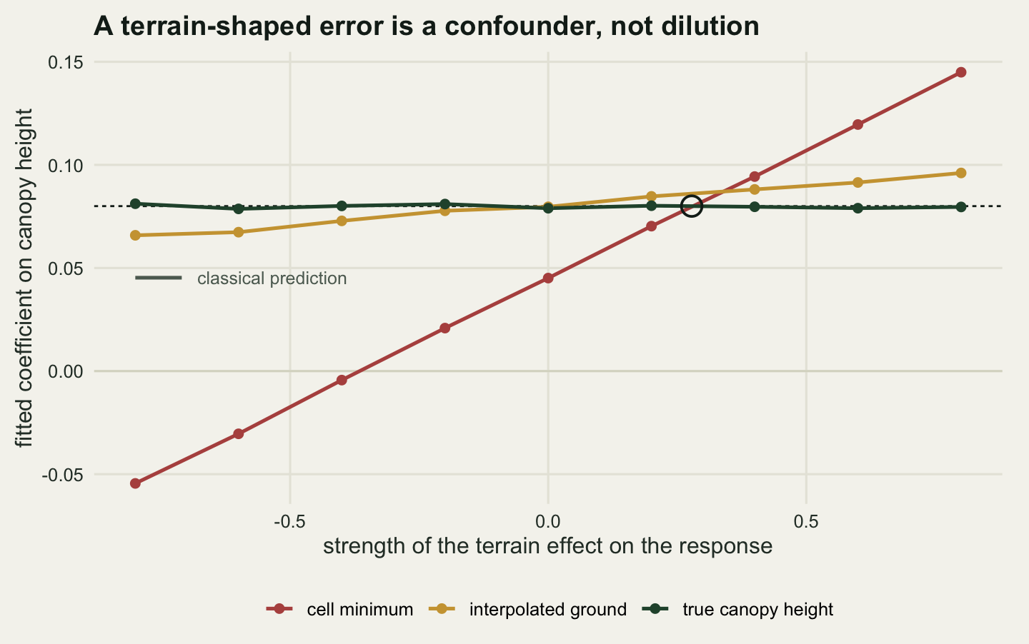
The interpolated covariate is better but not clean. It runs from 0.0659 to 0.0961 across the same sweep, a spread of 0.0302 against 0.1994 for the cell minimum, because it still carries the half window term from the previous section. The direction of the residual error is the same, and so is its cause.

What helps, and what each fix is worth

adj_spread <- max(coef_tab$adj_true) - min(coef_tab$adj_true)
dem_spread <- max(coef_tab$adj_dem) - min(coef_tab$adj_dem)
resid_var <- var(residuals(lm(chm_cm ~ terr)))
acc_claim <- 0.5
slope_probe <- c(10, 20, 25, 35)
max_cell <- acc_claim / tan(slope_probe * pi / 180)
gr_q1 <- unname(quantile(ngr_cell, 0.25))
bias_in <- chm_in - h_site
print(round(c(adjusted_spread = adj_spread, dem_adjusted_spread = dem_spread,
              naive_spread = max(coef_tab$cellmin) - min(coef_tab$cellmin),
              var_true_height = var(h_site),
              var_cellmin_after_terrain = resid_var), 4))

          adjusted_spread       dem_adjusted_spread              naive_spread 
                   0.0025                    0.0657                    0.1994 
          var_true_height var_cellmin_after_terrain 
                  15.9702                   15.7865 

print(rbind(slope_deg = slope_probe,
            largest_cell_metres = round(max_cell, 2)))

                     [,1]  [,2]  [,3]  [,4]
slope_deg           10.00 20.00 25.00 35.00
largest_cell_metres  2.84  1.37  1.07  0.71

print(round(c(lowest_quartile_ground_count = gr_q1,
              cor_count_bias = cor(ngr_cell, bias_in),
              bias_all_cells = mean(bias_in),
              bias_cells_kept = mean(bias_in[ngr_cell >= gr_q1]),
              bias_cells_dropped = mean(bias_in[ngr_cell < gr_q1])), 4))

lowest_quartile_ground_count               cor_count_bias 
                      7.7500                      -0.1264 
              bias_all_cells              bias_cells_kept 
                      0.4128                       0.2300 
          bias_cells_dropped 
                      0.9613 

Do not use a cell minimum. Switching to an interpolated surface at twenty-five degrees and a closure of 0.6 takes the bias from 9.03 metres to 0.756. That is the largest single improvement available and it costs nothing but a filter that every lidar toolchain already has.

Size the cell against the accuracy being claimed. The terrain drop inside a cell is \(c \tan\theta\), so a paper reporting canopy height to 0.5 metres on slopes of 25 degrees needs cells no wider than 1.07 metres for the cell minimum shortcut to be defensible, and 0.71 metres at 35 degrees. Those are not the cell sizes anyone uses. The claim, not the cell, is usually what has to give: at twenty metre cells and 20 degrees the terrain drop alone is 7.28 metres.

Count ground returns per cell and treat thin cells as missing. The count of returns classified as ground is an observable that comes free with the filter. As a continuous predictor of the error it is weak, correlating with the interpolated bias at only -0.126, because the bias also carries the slope term. As a screen it works: dropping the quartile of cells with fewer than 7.75 ground returns moves the mean bias of what remains from 0.4128 metres to 0.23, the discarded quartile carrying 0.9613, or 4.2 times as much. Treating those cells as missing is honest; treating them as measured puts the largest errors in the dataset next to the tallest stands.

Put the terrain in the model. Adding slope as a covariate alongside the biased height collapses the spread of the coefficient from 0.1994 to 0.0025 across the sweep, and the adjusted estimates average 0.0799 against a truth of 0.08. The adjustment works here because the bias is an exact function of the same slope used to correct it: the variance of the biased covariate that survives conditioning on slope is 15.79, against 15.97 for the true heights, so almost nothing but terrain was removed. Give the model a slope read off a coarse elevation model instead, with a few degrees of error, and the spread is 0.0657: better than 0.1994, and a long way from a fix. Report the slope distribution of the study area next to the height estimates either way, because a reader cannot judge any of this without it.

The honest limit

The terrain here is a plane. That is what makes the arithmetic checkable, and it is also the most favourable possible case for the interpolated normalisation, since a plane fitted through correct ground seeds is exactly right. Real terrain is convex on ridges and concave in hollows, and an interpolated surface built from sparse seeds cuts corners on both, which adds an error this simulation cannot show. Su and Bork (2006) measured elevation model error rising with both slope and vegetation on real ground, and Leitold et al (2015) found the terrain contribution to canopy height metrics in steep tropical forest large enough to change stand level biomass estimates. The numbers here are a lower bound on what curvature and roughness do.

The ground filter here is the first step of a filter rather than the whole of one. Kraus and Pfeifer (1998) iterate, reweighting points by their residual from the current surface, and a progressive triangulation adds points to a ground model only when they satisfy an angle and distance test. Both do better than a window minimum, particularly at recovering ground under scattered low vegetation. What neither can do is invent a ground return where no pulse reached the floor, so the density mechanism in the third section survives any improvement in the algorithm; what changes is the closure at which it starts to bite.

The canopy is uniform inside each cell. Real canopy height varies within twenty metres, and a cell maximum then reports the tallest tree rather than the stand, which is a separate upward bias that grows with cell size in the same direction as the terrain term. Splitting the two apart would need a crown level model and is a different post. The response model is also simpler than the one the scenario describes: a Gaussian response with independent errors, where a bird occupancy analysis would carry detection, spatial correlation between stations, and a link function. None of those changes the direction of the argument, because the covariate is wrong before the model sees it, but all of them change the size of what comes out.

Two things this post did not measure. Pulse density is held at 4 per square metre throughout, and both mechanisms depend on it: a denser survey finds the uphill corner of the cell more reliably, which makes the terrain bias worse, and finds more ground returns, which makes the density bias better. And scan angle is ignored entirely. Off-nadir pulses on a slope travel further through the canopy on the uphill side than the downhill side, which makes the whole geometry asymmetric in a way a plane and a vertical pulse cannot represent.

Where to go next

One check takes ten minutes on an analysis that is already finished. Pull the slope raster for the study area, plot the canopy height estimates against slope, and look at the sign of the relationship. If height rises with slope in a catchment where nobody expects taller trees on steeper ground, the covariate is carrying terrain. The second check is the ground return count per cell, which most toolchains will write out, and which should be reported as a map rather than a mean.

For the mechanics of building and reading the rasters involved, raster data in R with terra covers elevation models, slope and extraction at points, and from scattered plots to a surface covers the interpolation step that turns sparse ground seeds into a continuous surface, along with the variogram that says how far a seed’s information reaches. For the wider audit of a covariate that arrived from somebody else’s pipeline, checking a remote sensing covariate runs five checks of which this post is the long version of one. And measurement error and regression dilution is the case this one is not: read it for what a reliability ratio does when the error really is independent, then note that the correction it teaches would have pushed every coefficient in this post further from the truth.

References

Naesset E 2002 Remote Sensing of Environment 80(1):88-99 (10.1016/S0034-4257(01)00290-5)

Hyyppa J, Hyyppa H, Leckie D, Gougeon F, Yu X, Maltamo M 2008 International Journal of Remote Sensing 29(5):1339-1366 (10.1080/01431160701736489)

Vierling KT, Vierling LA, Gould WA, Martinuzzi S, Clawges RM 2008 Frontiers in Ecology and the Environment 6(2):90-98 (10.1890/070001)

Kraus K, Pfeifer N 1998 ISPRS Journal of Photogrammetry and Remote Sensing 53(4):193-203 (10.1016/S0924-2716(98)00009-4)

Sithole G, Vosselman G 2004 ISPRS Journal of Photogrammetry and Remote Sensing 59(1-2):85-101 (10.1016/j.isprsjprs.2004.05.004)

Reutebuch SE, McGaughey RJ, Andersen HE, Carson WW 2003 Canadian Journal of Remote Sensing 29(5):527-535 (10.5589/m03-022)

Gaveau DLA, Hill RA 2003 Canadian Journal of Remote Sensing 29(5):650-657 (10.5589/m03-023)

Su J, Bork EW 2006 Photogrammetric Engineering and Remote Sensing 72(11):1265-1274 (10.14358/PERS.72.11.1265)

Leitold V, Keller M, Morton DC, Cook BD, Shimabukuro YE 2015 Carbon Balance and Management 10(1):3 (10.1186/s13021-015-0013-x)

Related tutorials

• Checking a remote sensing covariate
• Raster data in R with terra: DEMs and extraction
• From scattered plots to a surface: IDW and kriging in R
• Measurement error and regression dilution