library(ggplot2)

te_pal <- list(forest = "#275139", green = "#2f8f63", sage = "#93a87f",
               clay = "#b5534e", gold = "#cda23f", line = "#dad9ca",
               ink = "#16241d", paper = "#f5f4ee")

theme_te <- function() {
  theme_minimal(base_size = 12) +
    theme(panel.grid.minor = element_blank(),
          panel.grid.major = element_line(colour = "#e7e6dc"),
          plot.background = element_rect(fill = "#f5f4ee", colour = NA),
          panel.background = element_rect(fill = "#f5f4ee", colour = NA),
          plot.title = element_text(face = "bold", colour = te_pal$ink),
          axis.title = element_text(colour = "#2c3a31"),
          axis.text = element_text(colour = "#2c3a31"),
          legend.position = "bottom")
}Splicing a monitoring series
R
monitoring
time series
trend
ecology tutorial
A method change part-way through a monitoring series manufactures a trend. Measuring the bias, the exchange rate per decade, and why no diagnostic fires.
A moth recording network runs twenty-four light traps, one per site, emptied every morning through the flight season, with the season’s catch of a common noctuid summed into one annual figure per trap. The series is twenty-eight years long. In its fifteenth year the mercury vapour bulbs were replaced with low-wattage actinic tubes across the whole network in a single winter, because the old bulbs had stopped being manufactured. Nothing else changed: the same sites, the same operators, the same season, the same species. The catches went on being written into the same column of the same spreadsheet.
A light trap does not sample a fixed volume of air. Merckx and Slade (2014) released marked moths at known distances from an actinic trap and recovered attraction radii differing by more than a factor of two between noctuids and the larger erebids, so what a trap draws in depends on the lamp as much as on the moths. Replacing the lamp was a change of instrument in the middle of a measurement series, and it left a step in the numbers. More than a decade later the network is asked whether the species is declining, and the analysis fits one line through twenty-eight annual values. Methodological change of exactly this kind is one of the reasons Didham et al (2020) give for treating published insect decline rates with care, and the wider problem of separating a signal of change from a change in how the recording was done runs through Isaac et al (2014).
The result of that fit is the subject of this post. A step at the seam reads as trend, the interval around the trend knows nothing about the seam, and none of the checks an analyst would ordinarily run has any purchase on it. The bias is not noise: the residuals are fine, the interval is narrow, the model is confident, and the answer is wrong by a quantity that can be worked out exactly from the size of the step and the length of the series.
This sits next to three posts and repeats none of them. Checking a monitoring design has a check on observer drift, but that drift is smooth: detection slipping by a fixed percentage every year, which adds a slope to a slope. A step is a different object and it behaves differently. That post also names the remedy in a single clause, that a subset of sites can be surveyed by a second method for calibration, and then carries none of it out: no code, no numbers, no idea what the calibration is worth. This post starts from that gap. Errors-in-variables and Deming regression supplies the calibration tool, but on a cross-sectional scatter of one method against another, with no time axis, no trend to protect and no question about how long the two methods have to run side by side. And segmented regression fits a break in a response along a covariate and treats the location of the break as the finding; here the break is in time, its year is written in the network’s protocol file, and the question is not where it is but whether anything in the data can see it at all.
Five measurements follow, all on synthetic counts with the generating trend known, so every error is a distance from a value that was set rather than an argument about what should have happened.
A network that changed its traps
The generating model is deliberately plain, because the point is what a plain analysis does to it. Each trap has its own catchability, every year has a weather effect shared across the network, each trap-year has its own departure from that, and the catch is Poisson around the resulting expectation. The population itself does not change: the true log-scale trend is set to zero. Then the new lamp multiplies every subsequent catch by a fixed factor.
The annual network index is the log of the mean catch per trap. Collapsing the twenty-four traps to one figure a year before fitting the trend is the standard move, and it is also the honest one: the weather effect is shared across traps, so treating trap-years as independent replicates for a trend test would put the error term at the wrong scale.
n_year <- 28
yr <- 1994:2021
t_c <- yr - mean(yr)
n_trap <- 24
sw_year <- 2008
new_era <- as.integer(yr >= sw_year)
k_old <- sum(new_era == 0)
beta_true <- 0
sd_trap <- 0.45
sd_year <- 0.22
sd_ty <- 0.35
mu_log <- log(60)
f_meth <- 0.72
step_log <- log(f_meth)

sim_series <- function(seed, step_sz = step_log, beta = beta_true) {
  set.seed(seed)
  a_i <- rnorm(n_trap, mu_log, sd_trap)
  u_t <- rnorm(n_year, 0, sd_year)
  e_it <- matrix(rnorm(n_trap * n_year, 0, sd_ty), n_trap, n_year)
  eta <- outer(a_i, rep(1, n_year)) +
    outer(rep(1, n_trap), beta * t_c + u_t) + e_it
  cnt_cl <- matrix(rpois(n_trap * n_year, exp(eta)), n_trap, n_year)
  cnt_sp <- matrix(rpois(n_trap * n_year,
                         exp(eta + rep(step_sz * new_era, each = n_trap))),
                   n_trap, n_year)
  list(clean = log(colMeans(cnt_cl)), spliced = log(colMeans(cnt_sp)))
}

print(c(years = n_year, traps = n_trap, changeover = sw_year,
        years_on_old_lamp = k_old, years_on_new_lamp = n_year - k_old,
        true_trend = beta_true, method_factor = f_meth))
years traps changeover years_on_old_lamp
28.00 24.00 2008.00 14.00
years_on_new_lamp true_trend method_factor
14.00 0.00 0.72 print(round(c(step_log_scale = step_log,
step_as_pct = 100 * (f_meth - 1),
mean_catch_old_lamp = exp(mu_log)), 4)) step_log_scale step_as_pct mean_catch_old_lamp
-0.3285 -28.0000 60.0000 The new lamp catches 28 per cent fewer moths than the old one, which on the log scale is a step of -0.3285. That factor is not extreme for a lamp change; it is the sort of difference a side-by-side trial would report and then nobody would apply.
d1 <- sim_series(20260731)

fit_tr <- function(idx) {
  m <- lm(idx ~ t_c)
  ci <- confint(m)
  c(slope = unname(coef(m)[2]),
    se = unname(summary(m)$coefficients[2, 2]),
    lo = ci[2, 1], hi = ci[2, 2],
    p = unname(summary(m)$coefficients[2, 4]),
    resid_sd = summary(m)$sigma)
}
one <- rbind(as_recorded = fit_tr(d1$clean), spliced = fit_tr(d1$spliced))
print(round(one, 5))
slope se lo hi p resid_sd
as_recorded -0.00873 0.00495 -0.01891 0.00146 0.08993 0.21179
spliced -0.02685 0.00583 -0.03883 -0.01488 0.00009 0.24910print(round(cbind(per_decade = 10 * one[, "slope"],
lo_decade = 10 * one[, "lo"],
hi_decade = 10 * one[, "hi"],
pct_decade = 100 * (exp(10 * one[, "slope"]) - 1)), 4)) per_decade lo_decade hi_decade pct_decade
as_recorded -0.0873 -0.1891 0.0146 -8.3576
spliced -0.2685 -0.3883 -0.1488 -23.5509On the series as recorded by one lamp throughout, the fitted trend is -0.0873 per decade on the log scale, interval -0.1891 to 0.0146, which contains zero, as it should. Splice the lamp change into the same underlying population and the fitted trend is -0.2685 per decade, interval -0.3883 to -0.1488. In the units a report would use, that is a decline of 23.551 per cent per decade with a p value of 0.000095, for a population that did not move.
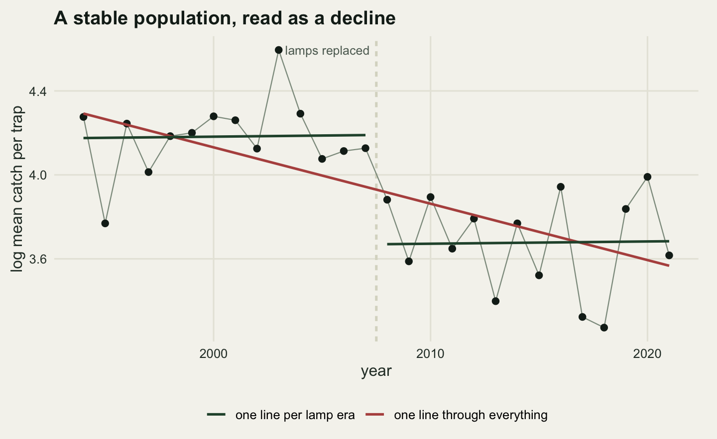
The bias is exact, and the interval does not notice it
One series proves nothing, so run two thousand. Each replicate redraws the trap effects, the weather, the trap-year departures and the Poisson counts, and fits the same one-line model to the series with the lamp change and to the series without it. Alongside the estimate, the loop stores the standard error, the residual standard deviation, the lag-one residual autocorrelation and a normality test, because those are the things an analyst would look at.
diag_of <- function(idx) {
  m <- lm(idx ~ t_c)
  r <- residuals(m)
  ci <- confint(m)
  c(slope = unname(coef(m)[2]),
    se = unname(summary(m)$coefficients[2, 2]),
    excl0 = as.numeric(ci[2, 1] * ci[2, 2] > 0),
    resid_sd = summary(m)$sigma,
    acf1 = sum(r[-1] * r[-length(r)]) / sum(r^2),
    dw = sum(diff(r)^2) / sum(r^2),
    shapiro_p = unname(shapiro.test(r)$p.value))
}

n_rep <- 2000
acc <- matrix(NA_real_, n_rep, 14)
for (b in seq_len(n_rep)) {
  dd <- sim_series(50000 + b)
  acc[b, ] <- c(diag_of(dd$clean), diag_of(dd$spliced))
}
nm_d <- c("slope", "se", "excl0", "resid_sd", "acf1", "dw", "shapiro_p")
colnames(acc) <- c(paste0("c_", nm_d), paste0("s_", nm_d))
acc <- as.data.frame(acc)

bias_pred <- step_log * 6 * k_old * (n_year - k_old) /
  (n_year * (n_year^2 - 1))
print(round(c(mean_slope_clean_dec = 10 * mean(acc$c_slope),
              mean_slope_spliced_dec = 10 * mean(acc$s_slope),
              predicted_bias_dec = 10 * bias_pred,
              predicted_pct_dec = 100 * (exp(10 * bias_pred) - 1)), 5))
mean_slope_clean_dec mean_slope_spliced_dec predicted_bias_dec
0.00216 -0.17408 -0.17621
predicted_pct_dec
-16.15573 print(round(c(mean_se_clean_dec = 10 * mean(acc$c_se),
mean_se_spliced_dec = 10 * mean(acc$s_se),
se_ratio = mean(acc$s_se) / mean(acc$c_se),
sd_slope_clean_dec = 10 * sd(acc$c_slope),
sd_slope_spliced_dec = 10 * sd(acc$s_slope),
sd_ratio = sd(acc$s_slope) / sd(acc$c_slope)), 5)) mean_se_clean_dec mean_se_spliced_dec se_ratio
0.05479 0.05833 1.06451
sd_slope_clean_dec sd_slope_spliced_dec sd_ratio
0.05588 0.05593 1.00074 print(round(c(excl_zero_clean = mean(acc$c_excl0),
excl_zero_spliced = mean(acc$s_excl0),
bias_in_se_units = (mean(acc$s_slope) - beta_true) /
mean(acc$s_se)), 4)) excl_zero_clean excl_zero_spliced bias_in_se_units
0.0495 0.8195 -2.9845 Over 2000 replicates the clean series averages 0.00216 per decade and the spliced one averages -0.17408, against a truth of 0. The predicted value is -0.17621, and the prediction is not a guess. For an ordinary least squares fit of the index on time, the coefficient on a step of size \(s\) entering at year \(k\) is
\[\text{bias} \;=\; s \cdot \frac{\operatorname{Cov}(\mathbb{1}[t > k],\, t)}{\operatorname{Var}(t)} \;=\; \frac{6\,s\,k\,(n-k)}{n\,(n^2-1)}\]
which depends on nothing except the step, the seam position and the series length. The population, the noise and the number of traps do not enter. In percentage terms the manufactured decline is 16.156 per cent per decade.
The second set of numbers is why this survives review. The mean standard error moves from 0.05479 per decade to 0.05833, a ratio of 1.0645: the reported precision worsens by 6.451 per cent while the estimate moves by 2.985 standard errors. The spread of the estimates across replicates barely changes either, 0.05588 per decade clean against 0.05593 spliced, a ratio of 1.0007. The whole sampling distribution slides sideways and keeps its shape, which is the definition of bias and the one thing a standard error cannot report.
The interval excludes zero in 4.95 per cent of clean replicates, which is the nominal rate, and in 81.95 per cent of spliced ones. Four networks in five would publish a significant decline in a population that never changed.
What a step is worth, in trend per decade
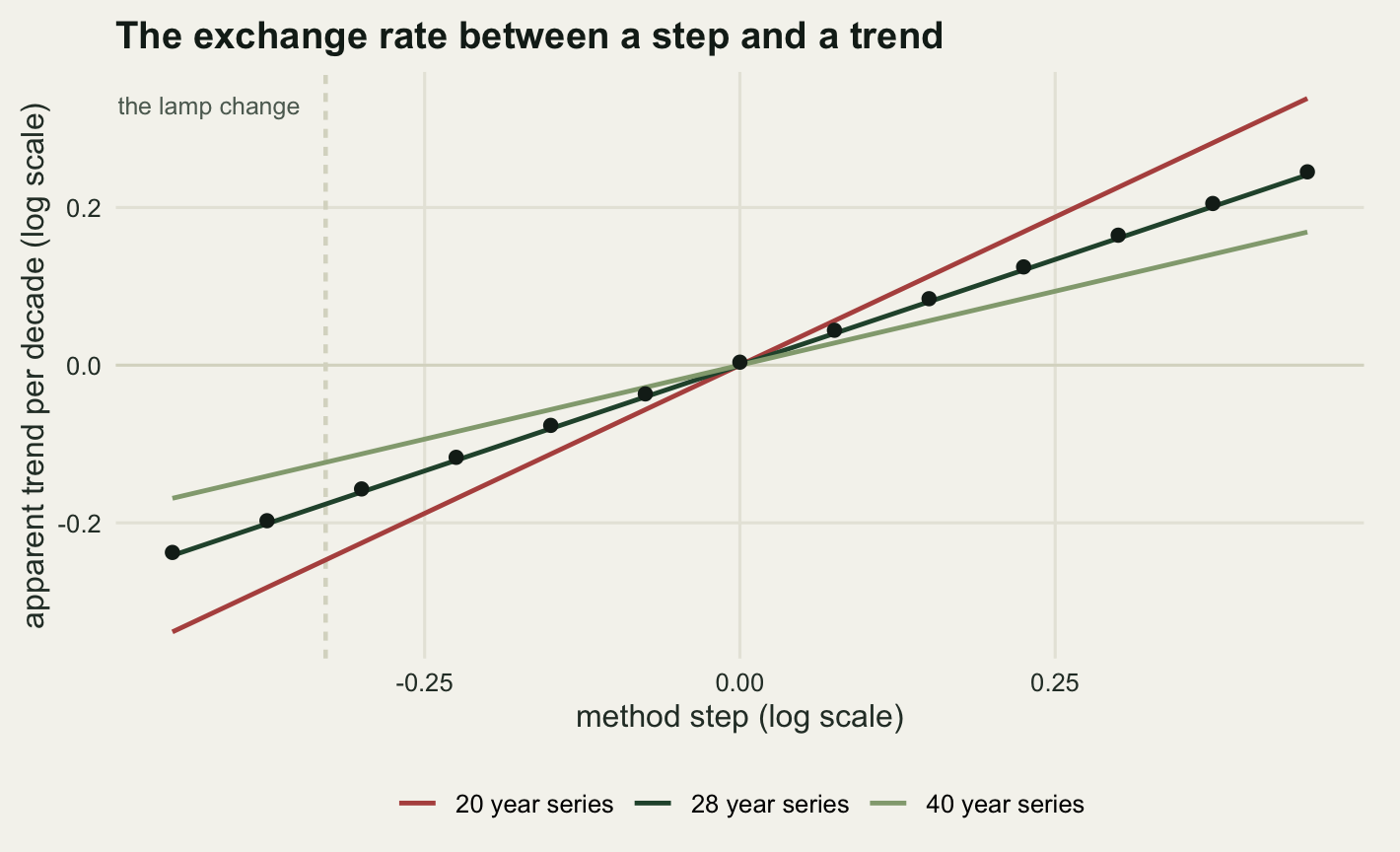
Since the bias depends only on three quantities, it can be quoted as an exchange rate: so much step buys so much trend. Sweeping the step over a range and measuring the mean fitted trend confirms the algebra and puts a number on the rate.
exch_rate <- function(nn, kk) 10 * 6 * kk * (nn - kk) / (nn * (nn^2 - 1))

step_grid <- seq(-0.45, 0.45, by = 0.075)
n_rep_x <- 400
ex_tab <- t(vapply(step_grid, function(s) {
  v <- numeric(n_rep_x)
  for (b in seq_len(n_rep_x)) {
    v[b] <- coef(lm(sim_series(80000 + b, step_sz = s)$spliced ~ t_c))[2]
  }
  c(step_log = s, pct_step = 100 * (exp(s) - 1), trend_dec = 10 * mean(v))
}, numeric(3)))
print(round(ex_tab, 5))
step_log pct_step trend_dec
[1,] -0.450 -36.23718 -0.23754
[2,] -0.375 -31.27107 -0.19730
[3,] -0.300 -25.91818 -0.15699
[4,] -0.225 -20.14838 -0.11689
[5,] -0.150 -13.92920 -0.07636
[6,] -0.075 -7.22565 -0.03643
[7,] 0.000 0.00000 0.00380
[8,] 0.075 7.78842 0.04429
[9,] 0.150 16.18342 0.08432
[10,] 0.225 25.23227 0.12464
[11,] 0.300 34.98588 0.16486
[12,] 0.375 45.49914 0.20507
[13,] 0.450 56.83122 0.24524xr_fit <- unname(coef(lm(ex_tab[, "trend_dec"] ~ ex_tab[, "step_log"] - 1))[1])
xr_theory <- exch_rate(n_year, k_old)
print(round(c(measured_exchange_rate = xr_fit,
closed_form_exchange_rate = xr_theory,
pct_per_decade_from_10pct_step =
100 * (exp(xr_theory * log(0.9)) - 1)), 5)) measured_exchange_rate closed_form_exchange_rate
0.53645 0.53640
pct_per_decade_from_10pct_step
-5.49479 len_grid <- c(15, 20, 28, 40, 60)
len_tab <- t(vapply(len_grid, function(nn) {
rr <- exch_rate(nn, nn %/% 2)
c(series_years = nn, exchange_rate = rr,
pct_dec_from_10pct_step = 100 * (exp(rr * log(0.9)) - 1),
fifteen_over_n = 15 / nn)
}, numeric(4)))
print(round(len_tab, 4)) series_years exchange_rate pct_dec_from_10pct_step fifteen_over_n
[1,] 15 1.0000 -10.0000 1.0000
[2,] 20 0.7519 -7.6162 0.7500
[3,] 28 0.5364 -5.4948 0.5357
[4,] 40 0.3752 -3.8764 0.3750
[5,] 60 0.2501 -2.6003 0.2500The measured exchange rate is 0.53645 against a closed form of 0.5364, agreeing to four decimal places. Read it in the direction a reader needs: a step of ten per cent in the index, placed in the middle of a twenty-eight year series, is worth 5.495 per cent per decade of apparent trend. That is a number to carry around. A protocol change nobody thought worth a footnote, a change small enough that a side-by-side trial might well have called it non-significant, buys close to a fifth of the thirty per cent per decade that puts a species in the Vulnerable category under IUCN criterion A2.
The rate falls as the series lengthens, and it falls roughly as fifteen over the number of years: 0.7519 at twenty years, 0.3752 at forty. A long series dilutes a fixed step, which is the one piece of good news here, and it is not much: doubling the length of a scheme halves the damage from a seam, and long schemes are the ones that have accumulated the most seams.
An era indicator buys back the trend and gives up the level
The repair is one term. Put an indicator for the lamp era into the model,
\[Y_t \;=\; \alpha + \beta\, t + \delta\, \mathbb{1}[t \geq \text{changeover}] + \varepsilon_t\]
and the step is absorbed by \(\delta\) while \(\beta\) carries the trend. Nothing is calibrated: no side-by-side trial, no conversion factor, no overlap period. The model is told only that the two halves are on different scales, not what the scales are.
To see that the trend really is recovered rather than merely shifted, the population now declines. The true log-scale trend is set to a real value and the same lamp step is applied on top of it.
beta_real <- -0.01
fit_pair <- function(idx) {
  m0 <- lm(idx ~ t_c)
  m1 <- lm(idx ~ t_c + new_era)
  c(naive = unname(coef(m0)[2]),
    naive_se = unname(summary(m0)$coefficients[2, 2]),
    era = unname(coef(m1)[2]),
    era_se = unname(summary(m1)$coefficients[2, 2]),
    delta = unname(coef(m1)[3]),
    delta_se = unname(summary(m1)$coefficients[3, 2]))
}
n_rep_e <- 2000
acc_e <- matrix(NA_real_, n_rep_e, 6)
for (b in seq_len(n_rep_e)) {
  acc_e[b, ] <- fit_pair(sim_series(70000 + b, beta = beta_real)$spliced)
}
colnames(acc_e) <- c("naive", "naive_se", "era", "era_se", "delta", "delta_se")
acc_e <- as.data.frame(acc_e)

t2 <- qt(0.975, n_year - 2)
t3 <- qt(0.975, n_year - 3)
print(round(c(true_trend_dec = 10 * beta_real,
              naive_mean_dec = 10 * mean(acc_e$naive),
              era_mean_dec = 10 * mean(acc_e$era),
              naive_bias_dec = 10 * (mean(acc_e$naive) - beta_real),
              era_bias_dec = 10 * (mean(acc_e$era) - beta_real)), 5))
true_trend_dec naive_mean_dec era_mean_dec naive_bias_dec era_bias_dec
-0.10000 -0.27773 -0.10188 -0.17773 -0.00188 print(round(c(naive_cover = mean(abs(acc_e$naive - beta_real) <
t2 * acc_e$naive_se),
era_cover = mean(abs(acc_e$era - beta_real) <
t3 * acc_e$era_se),
naive_se_dec = 10 * mean(acc_e$naive_se),
era_se_dec = 10 * mean(acc_e$era_se),
se_inflation = mean(acc_e$era_se) / mean(acc_e$naive_se),
sd_inflation = sd(acc_e$era) / sd(acc_e$naive)), 4)) naive_cover era_cover naive_se_dec era_se_dec se_inflation sd_inflation
0.1460 0.9540 0.0579 0.1090 1.8839 2.0003 print(round(c(delta_mean = mean(acc_e$delta), true_step = step_log,
delta_as_pct = 100 * (exp(mean(acc_e$delta)) - 1),
delta_detected = mean(abs(acc_e$delta / acc_e$delta_se) > t3)), 4)) delta_mean true_step delta_as_pct delta_detected
-0.3278 -0.3285 -27.9513 0.4090 The naive fit returns -0.2777 per decade against a truth of -0.1, and its nominal interval covers the truth 14.6 per cent of the time. With the era indicator the estimate is -0.1019 per decade, a bias of -0.00188, and coverage is 95.4 per cent. That is the practical lesson of the post, stated flatly: for a trend question the calibration is not needed. One dummy variable, costing one degree of freedom and no fieldwork, returns the trend unbiased.
What it costs is precision. The standard error goes from 0.0579 per decade to 0.109, and the honest measure of the cost is the spread of the estimates, which rises by a factor of 2.0003. That factor is not accidental. The era indicator and time are strongly collinear on a series split near its middle, and the variance inflation is \(1/(1 - R^2)\) where \(R^2 = 3k(n-k)/(n^2-1)\) is the fit of the step to a straight line in time. At a mid-series seam that gives a variance inflation of four and a spread multiplier of two, which is what came out.
What the model cannot do is put the two eras on one scale. The estimated step is -0.3278 on the log scale against a true -0.3285, so \(\delta\) is doing its job, but \(\delta\) is also only distinguishable from zero in 40.9 per cent of replicates. A question of the form “how many moths per trap now compared with the year the scheme started” has no answer from this model, because the answer would be the trend plus \(\delta\), and \(\delta\) is exactly the quantity nobody measured. Trend questions and level questions are not the same question, and only one of them survives a seam.
There is no safe place to put a seam
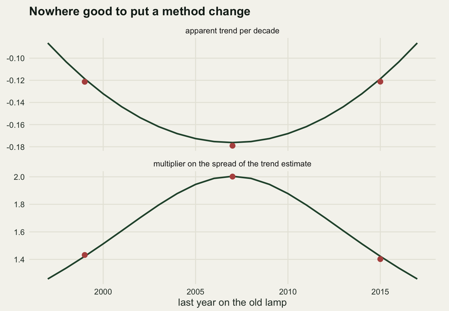
The bias formula and the variance inflation both depend on where in the series the changeover falls, and they pull in the same direction: the seam position that manufactures the most trend is also the position at which fixing it costs the most precision.
k_grid <- 4:(n_year - 4)
seam_tab <- data.frame(
  last_old_year = yr[k_grid],
  k = k_grid,
  bias_dec = step_log * exch_rate(n_year, k_grid),
  se_mult = 1 / sqrt(1 - 3 * k_grid * (n_year - k_grid) / (n_year^2 - 1)))
print(round(seam_tab[seq(1, nrow(seam_tab), by = 4), ], 4))
last_old_year k bias_dec se_mult
1 1997 4 -0.0863 1.2577
5 2001 8 -0.1438 1.6075
9 2005 12 -0.1726 1.9449
13 2009 16 -0.1726 1.9449
17 2013 20 -0.1438 1.6075
21 2017 24 -0.0863 1.2577check_k <- c(6, 14, 22)
n_rep_k <- 600
seam_chk <- t(vapply(check_k, function(kk) {
era_k <- as.integer(seq_len(n_year) > kk)
nb <- eb <- rr <- numeric(n_rep_k)
for (b in seq_len(n_rep_k)) {
set.seed(400000 + b)
a_i <- rnorm(n_trap, mu_log, sd_trap)
u_t <- rnorm(n_year, 0, sd_year)
e_it <- matrix(rnorm(n_trap * n_year, 0, sd_ty), n_trap, n_year)
eta <- outer(a_i, rep(1, n_year)) + outer(rep(1, n_trap), u_t) + e_it
cnt <- matrix(rpois(n_trap * n_year,
exp(eta + rep(step_log * era_k, each = n_trap))),
n_trap, n_year)
idx <- log(colMeans(cnt))
m0 <- lm(idx ~ t_c)
m1 <- lm(idx ~ t_c + era_k)
nb[b] <- 10 * coef(m0)[2]
eb[b] <- 10 * coef(m1)[2]
rr[b] <- summary(m1)$coefficients[2, 2] /
summary(m0)$coefficients[2, 2]
}
c(k = kk, sim_bias_dec = mean(nb),
theory_bias_dec = step_log * exch_rate(n_year, kk),
sim_era_dec = mean(eb), sim_sd_mult = sd(eb) / sd(nb),
sim_se_ratio = mean(rr),
theory_mult = 1 / sqrt(1 - 3 * kk * (n_year - kk) / (n_year^2 - 1)))
}, numeric(7)))
print(round(seam_chk, 4)) k sim_bias_dec theory_bias_dec sim_era_dec sim_sd_mult sim_se_ratio
[1,] 6 -0.1213 -0.1187 -0.0003 1.4320 1.3114
[2,] 14 -0.1791 -0.1762 -0.0021 2.0018 1.8872
[3,] 22 -0.1212 -0.1187 -0.0007 1.4021 1.3127
theory_mult
[1,] 1.4224
[2,] 2.0038
[3,] 1.4224worst <- seam_tab[which.max(abs(seam_tab$bias_dec)), ]
mild <- seam_tab[seam_tab$k == min(k_grid), ]
share <- abs(seam_tab$bias_dec) / max(abs(seam_tab$bias_dec))
print(round(c(worst_bias_dec = worst$bias_dec,
worst_se_mult = worst$se_mult,
earliest_seam_bias_dec = mild$bias_dec,
earliest_over_worst = mild$bias_dec / worst$bias_dec,
positions_above_80pct_of_worst = sum(share >= 0.8),
positions_tested = length(share)), 4)) worst_bias_dec worst_se_mult
-0.1762 2.0038
earliest_seam_bias_dec earliest_over_worst
-0.0863 0.4898
positions_above_80pct_of_worst positions_tested
13.0000 21.0000 At the worst position the manufactured trend is -0.1762 per decade and the era indicator multiplies the spread of the trend estimate by 2.0038. Move the changeover so that only four years sit on the old lamp, as early as this sweep goes, and the manufactured trend is still -0.0863 per decade, 48.98 per cent of the worst case. Across the 21 positions tested, 13 of them produce at least eighty per cent of the maximum bias.
That flatness is the finding. There is a folk intuition that a break near one end of a series is less of a problem, on the grounds that it affects only a few years. It affects only a few years and it still moves the trend by about half as much, because what matters is the covariance between the step and time, and that covariance is broad and blunt rather than sharply peaked. The three simulated positions agree with the algebra to within Monte Carlo error, and the era indicator returns essentially zero bias at all three.
One number in that table is smaller than the design algebra says it should be. At the mid-series seam the spread of the era-model estimates is 2.0018 times the spread of the naive ones, matching the predicted 2.0038, but the ratio of the reported standard errors is only 1.8872. The gap is the naive fit flattering itself: its residual standard deviation is inflated by the step it is failing to model, so part of the era indicator’s apparent cost has already been paid, invisibly, by the model that ignores the seam.
Why nothing in the output complains
The diagnostics were collected alongside the estimates in the replicate loop, so they can be read off directly. A step in the middle of a series does leave a residual pattern in principle: high residuals early, low residuals late, with a jump between. The question is whether that pattern is large enough to notice against the year-to-year variation of a real monitoring series.
q_acf <- unname(quantile(acc$c_acf1, 0.95))
q_dw <- unname(quantile(acc$c_dw, 0.05))
print(round(c(mean_acf1_clean = mean(acc$c_acf1),
              mean_acf1_spliced = mean(acc$s_acf1),
              clean_95th_acf1 = q_acf,
              spliced_above_that = mean(acc$s_acf1 > q_acf)), 4))
mean_acf1_clean mean_acf1_spliced clean_95th_acf1 spliced_above_that
-0.0766 0.0032 0.2223 0.1195 print(round(c(mean_dw_clean = mean(acc$c_dw),
mean_dw_spliced = mean(acc$s_dw),
clean_5th_dw = q_dw,
spliced_below_that = mean(acc$s_dw < q_dw)), 4)) mean_dw_clean mean_dw_spliced clean_5th_dw spliced_below_that
2.0866 1.9273 1.4947 0.1270 print(round(c(shapiro_rej_clean = mean(acc$c_shapiro_p < 0.05),
shapiro_rej_spliced = mean(acc$s_shapiro_p < 0.05),
median_p_clean = median(acc$c_shapiro_p),
median_p_spliced = median(acc$s_shapiro_p)), 4)) shapiro_rej_clean shapiro_rej_spliced median_p_clean median_p_spliced
0.0535 0.0470 0.5012 0.5122 print(round(c(resid_sd_clean = mean(acc$c_resid_sd),
resid_sd_spliced = mean(acc$s_resid_sd),
ci_width_ratio = mean(acc$s_se) / mean(acc$c_se)), 4)) resid_sd_clean resid_sd_spliced ci_width_ratio
0.2342 0.2493 1.0645 Lag-one residual autocorrelation moves from -0.0766 on the clean series to 0.0032 on the spliced one. That is a shift, and it is a shift from mildly negative to zero, which no analyst would look at twice. Judged against the clean distribution’s own upper five per cent point, the spliced series exceeds it 11.95 per cent of the time: a test at the five per cent level would flag about one series in eight. The Durbin-Watson statistic tells the same story, mean 2.0866 clean against 1.9273 spliced.
Normality is completely silent. Shapiro-Wilk rejects at the five per cent level in 5.35 per cent of clean replicates and 4.7 per cent of spliced ones, with median p values of 0.5012 and 0.5122. The residual standard deviation rises from 0.2342 to 0.2493, and that 6.451 per cent is the entire trace the step leaves in the fit’s own summary.
The one procedure that is built to see this is a changepoint scan. Fitting a level shift at a single, pre-specified year is the classical test for a break between two regressions (Chow 1960). When the year is not known in advance the test becomes a scan: fit the shift at every candidate year, take the largest F statistic, and compare it with the distribution of that maximum under no shift, because the break year is a parameter searched over rather than fixed (Andrews 1993). The critical value is simulated here from series generated with no step at all; the strucchange package implements the same family of tests with analytic critical values (Zeileis et al 2002).
cand <- 5:(n_year - 5)
X0 <- cbind(1, t_c)
q0 <- qr(X0)
d_til <- vapply(cand,
                function(kk) qr.resid(q0, as.numeric(seq_len(n_year) > kk)),
                numeric(n_year))
d_ss <- colSums(d_til^2)

sup_f <- function(y) {
  e0 <- qr.resid(q0, y)
  rss0 <- sum(e0^2)
  gain <- (as.vector(crossprod(d_til, e0))^2) / d_ss
  fv <- gain / ((rss0 - gain) / (n_year - 3))
  j <- which.max(fv)
  c(stat = fv[j], k = cand[j])
}

n_null <- 4000
null_f <- numeric(n_null)
for (b in seq_len(n_null)) {
  null_f[b] <- sup_f(sim_series(200000 + b, step_sz = 0)$clean)["stat"]
}
crit_f <- unname(quantile(null_f, 0.95))
print(round(c(median_null_supF = median(null_f), crit_95 = crit_f,
              naive_F_table_crit = qf(0.95, 1, n_year - 3),
              crit_ratio = crit_f / qf(0.95, 1, n_year - 3),
              candidates_searched = length(cand)), 4))
median_null_supF crit_95 naive_F_table_crit crit_ratio
3.8741 10.2017 4.2417 2.4051
candidates_searched
19.0000 det_grid <- sort(c(seq(0, 1, by = 0.1), -step_log))
n_rep_c <- 800
det_tab <- t(vapply(det_grid, function(s) {
hit <- 0
near <- 0
for (b in seq_len(n_rep_c)) {
fv <- sup_f(sim_series(300000 + b, step_sz = -s)$spliced)
if (fv["stat"] > crit_f) hit <- hit + 1
if (abs(fv["k"] - k_old) <= 1) near <- near + 1
}
c(step_log = s, pct_step = 100 * (1 - exp(-s)),
detect = hit / n_rep_c, break_within_one_year = near / n_rep_c,
trend_dec = -s * exch_rate(n_year, k_old))
}, numeric(5)))
print(round(det_tab, 4)) step_log pct_step detect break_within_one_year trend_dec
[1,] 0.0000 0.0000 0.0462 0.2087 0.0000
[2,] 0.1000 9.5163 0.0575 0.2362 -0.0536
[3,] 0.2000 18.1269 0.0900 0.3412 -0.1073
[4,] 0.3000 25.9182 0.1550 0.4888 -0.1609
[5,] 0.3285 28.0000 0.1875 0.5337 -0.1762
[6,] 0.4000 32.9680 0.2788 0.6388 -0.2146
[7,] 0.5000 39.3469 0.4512 0.7725 -0.2682
[8,] 0.6000 45.1188 0.6562 0.8738 -0.3218
[9,] 0.7000 50.3415 0.7938 0.9238 -0.3755
[10,] 0.8000 55.0671 0.8862 0.9700 -0.4291
[11,] 0.9000 59.3430 0.9625 0.9912 -0.4828
[12,] 1.0000 63.2121 0.9875 0.9950 -0.5364mono <- cummax(det_tab[, "detect"])
inc <- which(!duplicated(mono))
need <- approx(mono[inc], det_tab[inc, "step_log"], xout = c(0.5, 0.8))$y
work <- det_tab[which.min(abs(det_tab[, "step_log"] + step_log)), ]
print(round(c(detect_at_lamp_step = unname(work["detect"]),
step_for_50pct = need[1], step_for_80pct = need[2],
pct_step_for_50 = 100 * (1 - exp(-need[1])),
pct_step_for_80 = 100 * (1 - exp(-need[2])),
trend_dec_at_50 = -need[1] * exch_rate(n_year, k_old),
trend_dec_at_80 = -need[2] * exch_rate(n_year, k_old)), 4))detect_at_lamp_step step_for_50pct step_for_80pct pct_step_for_50
0.1875 0.5238 0.7068 40.7723
pct_step_for_80 trend_dec_at_50 trend_dec_at_80
50.6759 -0.2810 -0.3791 The simulated critical value is 10.202, against 4.242 from the F table that a naive application would use: searching over 19 candidate years multiplies the threshold by 2.405, and ignoring that is how a scan of this kind manufactures its own false positives.
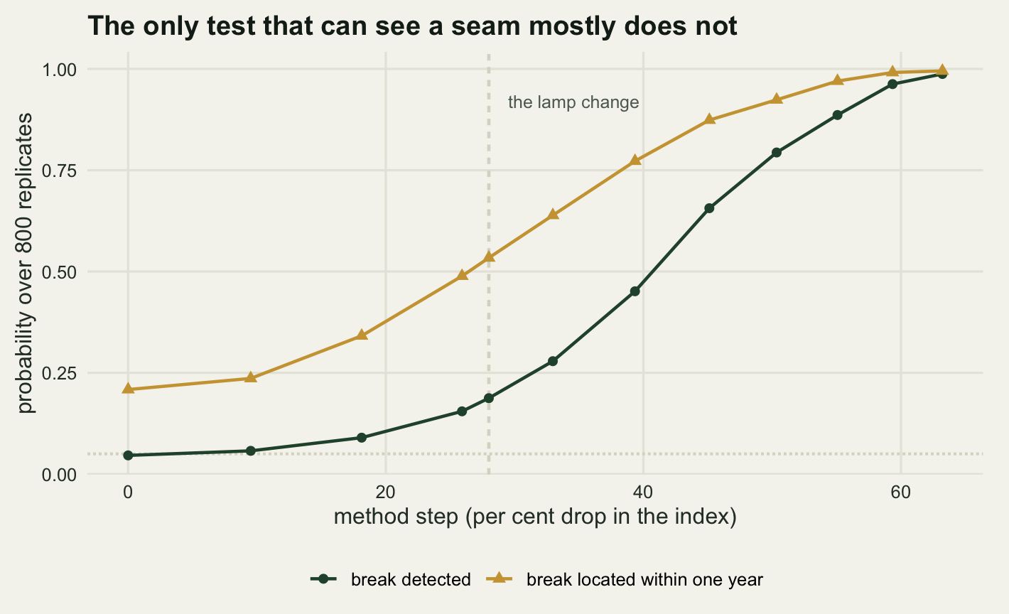
At the lamp step actually in play, the scan detects the break in 18.75 per cent of series. It reaches a coin flip at a step of 0.5238, a drop of 40.77 per cent, and four times in five at 0.7068, a drop of 50.68 per cent. By the time the scan is reliable the step is already manufacturing a trend of -0.3791 per decade, which is 31.55 per cent per decade. The test becomes trustworthy at exactly the sizes where the damage is beyond argument, and it is quiet across the whole range where the damage is merely serious.
The limit: a step and an abrupt change are the same data
Everything above treated the step as an artefact because the simulation was told it was one. Take that away and the problem stops being statistical. Consider two networks. In the first the population is stable and the lamps were replaced in the changeover year. In the second the lamps were never touched and the population really did drop, in one bad winter, by exactly the factor the lamp change would have produced.
n_tr_big <- 400
n_yr_big <- 80

two_stories <- function(seed, n_tr, n_yv) {
  set.seed(seed)
  tv <- seq_len(n_yv) - mean(seq_len(n_yv))
  era_v <- as.integer(seq_len(n_yv) > n_yv %/% 2)
  a_i <- rnorm(n_tr, mu_log, sd_trap)
  u_t <- rnorm(n_yv, 0, sd_year)
  e_it <- matrix(rnorm(n_tr * n_yv, 0, sd_ty), n_tr, n_yv)
  base_eta <- outer(a_i, rep(1, n_yv)) + outer(rep(1, n_tr), u_t) + e_it

  pop_stable <- rep(0, n_yv)                 # the population never moves
  pop_crashed <- step_log * era_v            # one bad winter, then stable
  lamps_swapped <- step_log * era_v          # the instrument step
  lamps_kept <- rep(0, n_yv)                 # no instrument change

  eta_method <- base_eta + rep(pop_stable + lamps_swapped, each = n_tr)
  eta_ecology <- base_eta + rep(pop_crashed + lamps_kept, each = n_tr)
  cnt <- matrix(rpois(n_tr * n_yv, exp(eta_method)), n_tr, n_yv)
  list(gap = max(abs(eta_method - eta_ecology)),
       same = identical(eta_method, eta_ecology),
       index = log(colMeans(cnt)), tv = tv, era = era_v)
}

small <- two_stories(20260732, n_trap, n_year)
large <- two_stories(20260733, n_tr_big, n_yr_big)
print(c(small_expectations_identical = small$same,
        large_expectations_identical = large$same))
small_expectations_identical large_expectations_identical
TRUE TRUE print(c(small_max_gap = small$gap, large_max_gap = large$gap,
large_traps = n_tr_big, large_years = n_yr_big))small_max_gap large_max_gap large_traps large_years
0 0 400 80 n_rep_i <- 1000
acc_i <- matrix(NA_real_, n_rep_i, 2)
for (b in seq_len(n_rep_i)) {
mi <- lm(sim_series(90000 + b)$spliced ~ t_c + new_era)
acc_i[b, ] <- c(10 * coef(mi)[2], coef(mi)[3])
}
print(round(c(era_trend_dec = mean(acc_i[, 1]),
mc_se_trend = sd(acc_i[, 1]) / sqrt(n_rep_i),
era_step = mean(acc_i[, 2]),
mc_se_step = sd(acc_i[, 2]) / sqrt(n_rep_i),
true_step = step_log,
step_as_pct = 100 * (exp(mean(acc_i[, 2])) - 1),
naive_trend_dec = 10 * mean(acc$s_slope)), 4)) era_trend_dec mc_se_trend era_step mc_se_step true_step
-0.0016 0.0036 -0.3244 0.0058 -0.3285
step_as_pct naive_trend_dec
-27.7056 -0.1741 The two stories are written down differently and they put the same expectation into every trap-year, so identical() on the two expectation matrices returns TRUE and the largest discrepancy is 0. Raise the network to 400 traps and 80 years and it is still 0. There is no statistic to compute, because there is nothing to compute it on: the two hypotheses are one distribution, and no test has power against a difference that does not exist.
The sting is in what that does to the era model. Averaged over 1000 networks it returns a trend of -0.00157 per decade, Monte Carlo standard error 0.00358, and a step of -0.3244 against a true -0.3285, which is a drop of 27.706 per cent. It is the right model under both stories, and what differs is which coefficient counts as ecology. Under the lamp story, \(\delta\) is an artefact to be discarded and the trend is the finding; under the bad-winter story, \(\delta\) is the finding and the flat trend either side of it is the finding too. Same data, same fit, opposite reports. The one thing that is definitely wrong under both stories is the single straight line, which puts -0.17408 per decade of steady decline into a network that was either stable throughout or stable, dropped once and stable again.
So the distinction is documentary. It lives in the network’s protocol file, in the equipment purchase records, in whatever somebody wrote down in the winter of the changeover, and there is no amount of data that substitutes for it. The practical consequence is small and dull: a column in the database recording which method produced each row, maintained from the first year, costs nothing and is the only thing that makes the era indicator legitimate rather than an assumption.
Observer turnover is the same object under a different name, and the schemes that took it seriously did exactly that. The North American Breeding Bird Survey carries observer identity in its database, which is what allowed between-observer differences in counts to be measured (Sauer, Peterjohn and Link 1994) and a distinct first-year effect for new observers to be separated from them (Kendall, Peterjohn and Sauer 1996). Neither result could have been recovered from the counts alone. A method column is the same idea applied to the instrument rather than the person.
What to take away
A method change part-way through a series is a bias, and bias is the failure mode that monitoring statistics is worst at reporting. The lamp change here moved the fitted trend by -0.17621 per decade, 2.985 standard errors, while widening the reported interval by 6.451 per cent and leaving the spread of the estimate across replicates unchanged at a ratio of 1.0007. Four fifths of such networks would report a significant decline in a stable population.
The exchange rate is the number to remember. At a mid-series seam, apparent trend per decade is 0.5364 times the log step, so a ten per cent step buys 5.495 per cent per decade over twenty-eight years, and the rate scales as roughly fifteen over the number of years. Two things about the seam position went against what I expected. The bias curve is nearly flat across the middle of the series, 13 of 21 tested positions producing at least eighty per cent of the maximum, so there is no end of the series where a seam is cheap. And the position that manufactures the most trend is also the one where the repair costs most: at mid-series the era indicator multiplies the spread of the estimate by 2.0038, the collinearity between a half-and-half step and a straight line being at its worst exactly there.
The repair itself is cheaper than the literature’s usual advice implies. An era indicator recovered a real trend of -0.1 per decade as -0.1019 with 95.4 per cent coverage, using no calibration data at all. It gives up the level, and it gives up 2.0003 times the precision, and for a trend question those are the right things to give up.
The diagnostics deserve one line each because that is all they earn. Normality: silent. Residual standard deviation: 6.451 per cent higher. Lag-one autocorrelation: flags 11.95 per cent of spliced series against a nominal five. A changepoint scan is the only thing that looks for the right object, and at the step in play it found it 18.75 per cent of the time, needing a 50.68 per cent step before it worked four times in five.
The honest limit is that none of this identifies the seam from inside the data. A method step and a genuine abrupt change generate the same distribution, to the last digit at any number of traps and any number of years, and the era model that fits both cannot say which of its two coefficients is the ecology. That is a documentation problem rather than a statistical one. The remaining question is the one this post deliberately did not ask: if the network had run both lamps side by side for a few seasons, how many seasons would it have taken to buy back the precision the era indicator throws away? That is measured in how long a calibration overlap, which treats the seam as a design decision rather than an accident.
References
Chow GC 1960 Econometrica 28(3):591-605 (10.2307/1910133)
Andrews DWK 1993 Econometrica 61(4):821-856 (10.2307/2951764)
Zeileis A, Leisch F, Hornik K, Kleiber C 2002 Journal of Statistical Software 7(2):1-38 (10.18637/jss.v007.i02)
Sauer JR, Peterjohn BG, Link WA 1994 The Auk 111(1):50-62 (10.2307/4088504)
Kendall WL, Peterjohn BG, Sauer JR 1996 The Auk 113(4):823-829 (10.2307/4088860)
Merckx T, Slade EM 2014 Insect Conservation and Diversity 7(5):453-461 (10.1111/icad.12068)
Didham RK, et al 2020 Insect Conservation and Diversity 13(2):103-114 (10.1111/icad.12408)
Isaac NJB, van Strien AJ, August TA, de Zeeuw MP, Roy DB 2014 Methods in Ecology and Evolution 5(10):1052-1060 (10.1111/2041-210X.12254)