library(ggplot2)

te_pal <- list(forest = "#275139", green = "#2f8f63", sage = "#93a87f",
               clay = "#b5534e", gold = "#cda23f", line = "#dad9ca",
               ink = "#16241d", paper = "#f5f4ee")

theme_te <- function() {
  theme_minimal(base_size = 12) +
    theme(panel.grid.minor = element_blank(),
          panel.grid.major = element_line(colour = "#e7e6dc"),
          plot.background = element_rect(fill = "#f5f4ee", colour = NA),
          panel.background = element_rect(fill = "#f5f4ee", colour = NA),
          plot.title = element_text(face = "bold", colour = te_pal$ink),
          axis.title = element_text(colour = "#2c3a31"),
          axis.text = element_text(colour = "#2c3a31"),
          legend.position = "bottom")
}How long a calibration overlap do you need?
R
monitoring
survey design
time series
ecology tutorial
A monitoring scheme is about to change method. Measuring how many years of dual running buy back the trend, and when a free era indicator is the better spend.
The same moth recording network as the previous post, at an earlier moment. Twenty-four light traps, one per site, emptied every morning through the flight season, with the season’s catch of a common noctuid summed into one annual figure per trap. The series is fourteen years old and the scheme intends to run it for at least as long again. This winter a letter arrived from the supplier: the mercury vapour bulbs are being discontinued, and from next season the network will have to run low-wattage actinic tubes instead.
The scheme has a small budget for the changeover, and one obvious thing to spend it on. Some traps can run both lamps for a few seasons before the old bulbs are retired, and the pairs of catches would fix the conversion between the two instruments. Whether that is worth doing, and for how many seasons at how many traps, is a design question with a numerical answer, and it has to be answered before the last mercury vapour bulb burns out. What is being bought is not obvious either. A light trap does not sample a fixed volume of air, and the two lamps differ across the spectrum in ways that different moths respond to differently: Merckx and Slade (2014) recovered attraction radii differing by more than a factor of two between macro-moth families at one lamp, Infusino et al (2017) found UV LED traps comparable with mercury vapour for some assemblages and not others, and van Grunsven et al (2014) showed that the available spectral response models predict the differences between lamp types poorly. So the conversion is real, it is not a physical constant, and the trial is the only way to see it. Networks of exactly this shape produced the evidence for steep declines in common and widespread British moths (Conrad et al 2006), and the difficulty of telling a change in a population from a change in how it was recorded runs through Isaac et al (2014).
This post measures four things: what a year of dual running is worth in trend precision, how that compares with spending the same observer-days on more survey years, how much the composition of the trial matters as against its length, and what happens to the reported interval when the conversion is treated as known. It is the design half of a pair. Splicing a monitoring series is the diagnosis: it takes the same network after an unplanned changeover, measures the trend the seam manufactures, and shows that an era indicator in the model recovers the trend with no calibration data at all. That result is the benchmark here, because a trial has to beat a free dummy variable before it is worth a single observer-night. Checking a monitoring design names a calibration subset in one clause and carries none of it out. Errors-in-variables and Deming regression supplies the two-method calibration tool on a cross-sectional scatter, with no time axis and no trend to protect. And power to detect a population trend asks whether a fixed budget is better spent on sites or on years; the calibration overlap is a third thing to spend it on, and it is compared against the other two below.
The design and the quantity the trial has to estimate
The generating model is the one from the companion post with one addition. Each trap has its own catchability, every year has a weather effect shared across the network, each trap-year has its own departure, and the catch is Poisson around the result. The population declines at a set rate. The new lamp multiplies the catch by a factor, and that factor is not the same at every trap: it depends on how rich the trap is, because a richer trap loses relatively more when the lamp changes.
n_year <- 28
yr <- 1994:2021
t_c <- yr - mean(yr)
n_trap <- 24
sw_year <- 2008
new_era <- as.integer(yr >= sw_year)
k_old <- sum(new_era == 0)
beta_true <- -0.01
sd_trap <- 0.45
sd_year <- 0.22
sd_ty <- 0.35
mu_log <- log(60)
f_meth <- 0.72
step_log <- log(f_meth)
gam_c <- -0.30
ov_max <- 12
ov_cols <- (k_old - ov_max + 1):k_old
xr_yr <- 6 * k_old * (n_year - k_old) / (n_year * (n_year^2 - 1))
n_ext <- 2
n_long <- n_year + n_ext
yr_l <- 1994:(1993 + n_long)
t_l <- yr_l - mean(yr_l)
era_l <- as.integer(yr_l >= sw_year)
budget <- 48
as_pct <- function(x) 100 * (1 - exp(-x))

print(c(traps = n_trap, years = n_year, changeover = sw_year,
        old_lamp_years = k_old, true_trend_per_decade = 10 * beta_true))
traps years changeover
24.0 28.0 2008.0
old_lamp_years true_trend_per_decade
14.0 -0.1 print(round(c(method_factor = f_meth, step_log = step_log,
conversion_sd_across_traps = abs(gam_c) * sd_trap,
exchange_rate_per_decade = 10 * xr_yr), 4)) method_factor step_log
0.7200 -0.3285
conversion_sd_across_traps exchange_rate_per_decade
0.1350 0.5364 The quantity that decides everything is the exchange rate between a residual step and an apparent trend, derived in the companion post: for a seam at year \(k\) of an \(n\) year series, an uncorrected step of size \(s\) in the index moves the fitted trend by \(6sk(n-k)/(n(n^2-1))\). Here that is 0.5364 per decade for every unit of log step left behind. A calibration does not have to be perfect, then; it has to leave a residue small enough that 0.5364 times it is small next to the precision the series already has. That single multiplier is what turns a field budget into a statistical answer.
The trial estimates a network-level conversion, and that is a slightly different thing from the per-trap conversion. The network index is the log of the mean catch per trap, so what has to be removed from it is the log ratio of the network total under the two lamps, which weights each trap by its catch.
sim_net <- function(seed, beta = beta_true, gam = gam_c, n_yv = n_long) {
  set.seed(seed)
  tv <- (1:n_yv) - mean(1:n_yv)
  era_v <- as.integer(seq_len(n_yv) > k_old)
  a_i <- rnorm(n_trap, mu_log, sd_trap)                 # trap catchability
  c_i <- gam * (a_i - mu_log)                           # conversion varies with it
  u_t <- rnorm(n_yv, 0, sd_year)                        # weather, shared
  base <- outer(a_i, rep(1, n_yv)) + outer(rep(1, n_trap), beta * tv + u_t)
  cnt <- matrix(rpois(n_trap * n_yv,
                      exp(base + matrix(rnorm(n_trap * n_yv, 0, sd_ty),
                                        n_trap, n_yv) +
                            outer(c_i + step_log, era_v))), n_trap, n_yv)
  # the dual-run catches: same trap, same year, own trap-year departure
  new_ov <- matrix(rpois(n_trap * ov_max,
                         exp(base[, ov_cols] +
                               matrix(rnorm(n_trap * ov_max, 0, sd_ty),
                                      n_trap, ov_max) +
                               (c_i + step_log))), n_trap, ov_max)
  list(idx = log(colMeans(cnt))[seq_len(n_year)],
       idx_long = log(colMeans(cnt)), u_t = u_t, a_i = a_i,
       d_star = step_log + log(sum(exp(a_i + c_i))) - log(sum(exp(a_i))),
       new_ov = new_ov, old_ov = cnt[, ov_cols, drop = FALSE])
}

conv_est <- function(z, traps, k) {                     # ratio of the two totals
  cc <- (ov_max - k + 1):ov_max
  log(sum(z$new_ov[traps, cc])) - log(sum(z$old_ov[traps, cc]))
}
tr_slope <- function(y) unname(coef(lm(y ~ t_c))[2])
rmse_dec <- function(x) 10 * sqrt(mean((x - beta_true)^2))

z1 <- sim_net(20260801)
print(round(c(true_network_step = z1$d_star, nominal_step = step_log,
              gap = z1$d_star - step_log), 4))
true_network_step nominal_step gap
-0.3766 -0.3285 -0.0481 In this network the true network step is -0.3766 against a nominal per-trap factor of -0.3285, a gap of -0.0481 produced entirely by the richest traps losing the most. That gap is worth 0.0258 per decade on its own, which is the first sign that what the trial is asked to estimate needs saying precisely before it is estimated at all.
The trial itself runs in the last few seasons before the changeover: a subset of traps is worked with both lamps, on separate nights, so the two catches share the trap and the year but not the night-to-night departure. Running the old lamp on for a few seasons after the changeover instead gives the same information and the same arithmetic.
What a year of dual running buys
Six of the twenty-four traps run both lamps, for between one and twelve seasons. For each replicate network the loop fits four things: the naive splice, the era indicator, the calibrated splice at each overlap length, and, as a floor, the splice corrected by the true network step. It records the trend error and the error in a level question, defined as the change in the index between the first and last year of the series, which is what a report means by asking how the network compares with when it started.
n_rep <- 2000
ov_len <- 0:12
n_dual <- 6
sw_tr <- matrix(NA_real_, n_rep, length(ov_len))
sw_lv <- sw_tr
sw_dd <- sw_tr
era_tr <- nai_tr <- perf_tr <- era_lv <- nai_lv <- numeric(n_rep)
for (b in seq_len(n_rep)) {
  z <- sim_net(600000 + b)
  tru_lv <- beta_true * (t_c[n_year] - t_c[1]) + z$u_t[n_year] - z$u_t[1]
  obs_lv <- z$idx[n_year] - z$idx[1]
  nai_tr[b] <- tr_slope(z$idx)
  nai_lv[b] <- obs_lv - tru_lv
  perf_tr[b] <- tr_slope(z$idx - z$d_star * new_era)
  m_era <- lm(z$idx ~ t_c + new_era)
  era_tr[b] <- unname(coef(m_era)[2])
  era_lv[b] <- obs_lv - unname(coef(m_era)[3]) - tru_lv
  for (j in seq_along(ov_len)) {
    if (ov_len[j] == 0) {
      sw_tr[b, j] <- nai_tr[b]
      sw_lv[b, j] <- nai_lv[b]
      next
    }
    dh <- conv_est(z, seq_len(n_dual), ov_len[j])
    sw_dd[b, j] <- dh - z$d_star
    sw_tr[b, j] <- tr_slope(z$idx - dh * new_era)
    sw_lv[b, j] <- obs_lv - dh - tru_lv
  }
}

sweep_tab <- data.frame(
  overlap_years = ov_len,
  dual_trap_years = ov_len * n_dual,
  conv_sd = apply(sw_dd, 2, sd),
  trend_mse = apply(sw_tr, 2, function(x) mean((x - beta_true)^2)),
  trend_rmse_dec = apply(sw_tr, 2, rmse_dec),
  pct_dec = as_pct(apply(sw_tr, 2, rmse_dec)),
  level_rmse = sqrt(colMeans(sw_lv^2)))
print(round(sweep_tab, 5))
overlap_years dual_trap_years conv_sd trend_mse trend_rmse_dec pct_dec
1 0 0 NA 0.00044 0.20942 18.89423
2 1 6 0.23686 0.00019 0.13949 13.02011
3 2 12 0.17304 0.00012 0.10936 10.35910
4 3 18 0.14553 0.00009 0.09663 9.21084
5 4 24 0.12883 0.00008 0.08861 8.47987
6 5 30 0.11828 0.00007 0.08444 8.09758
7 6 36 0.11090 0.00007 0.08164 7.83941
8 7 42 0.10466 0.00006 0.07882 7.57948
9 8 48 0.09906 0.00006 0.07670 7.38306
10 9 54 0.09479 0.00006 0.07492 7.21805
11 10 60 0.09184 0.00005 0.07376 7.11080
12 11 66 0.08926 0.00005 0.07276 7.01792
13 12 72 0.08675 0.00005 0.07173 6.92170
level_rmse
1 0.39837
2 0.26779
3 0.20881
4 0.18763
5 0.17333
6 0.16568
7 0.16049
8 0.15599
9 0.15264
10 0.14964
11 0.14786
12 0.14651
13 0.14530era_rmse <- rmse_dec(era_tr)
perf_rmse <- rmse_dec(perf_tr)
print(round(c(era_trend_rmse_dec = era_rmse,
era_level_rmse = sqrt(mean(era_lv^2)),
naive_trend_rmse_dec = rmse_dec(nai_tr),
naive_level_rmse = sqrt(mean(nai_lv^2)),
conversion_known_rmse_dec = perf_rmse), 5)) era_trend_rmse_dec era_level_rmse naive_trend_rmse_dec
0.11343 0.22623 0.20942
naive_level_rmse conversion_known_rmse_dec
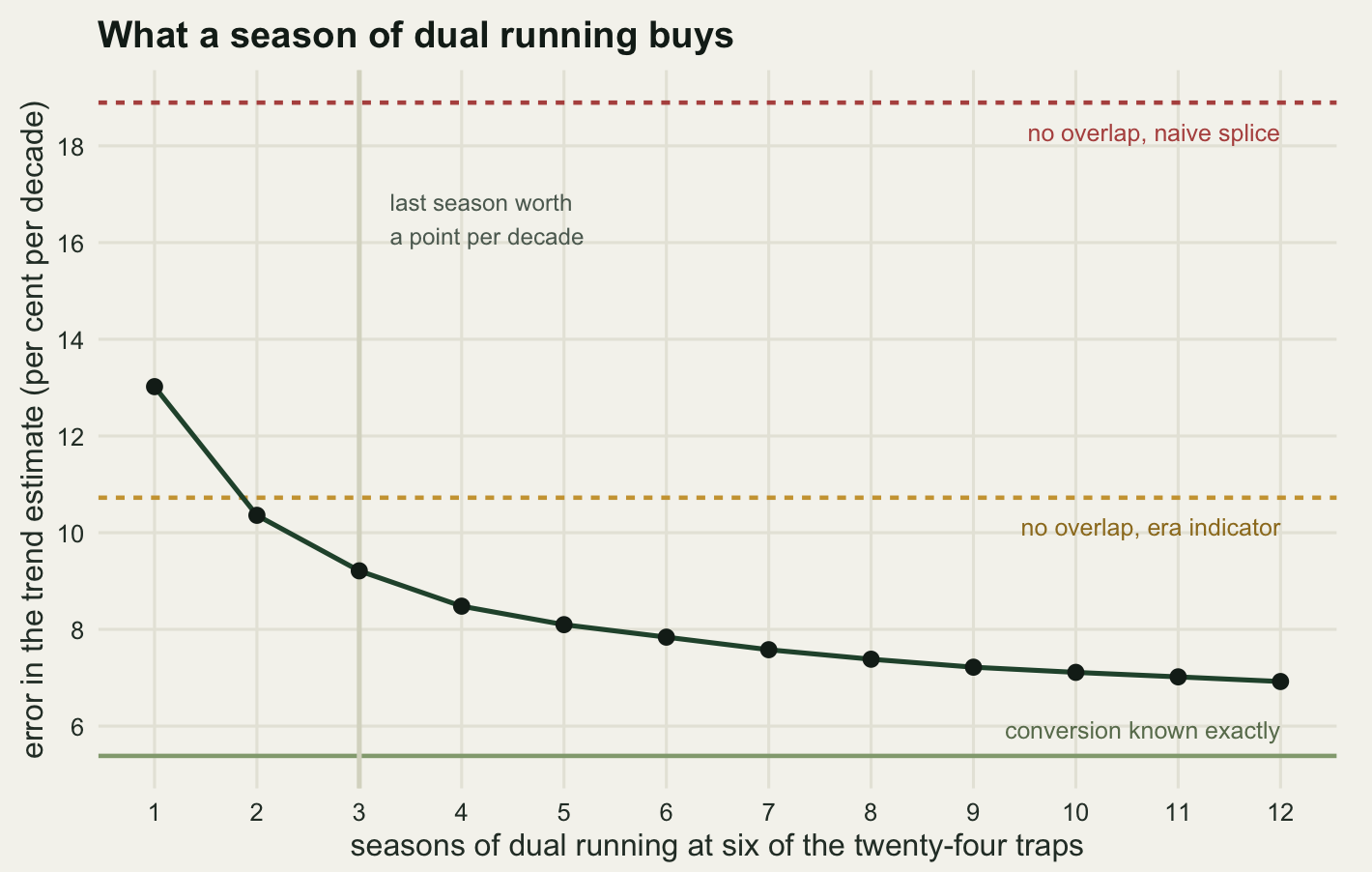
0.39837 0.05533 Three reference points before the curve. The naive splice, which subtracts nothing, has a trend error of 18.89 per cent per decade, almost all of it bias. The era indicator, which costs nothing, has 10.72. And a splice corrected by the true conversion, which no trial can achieve, has 5.38. Overlap lengths of two seasons and up live between the second and the third of those; a single season sits above the era indicator, and the first is the reason anyone is having this conversation.
pred_rmse <- sqrt(perf_rmse^2 + (10 * xr_yr * sweep_tab$conv_sd)^2)
print(round(cbind(overlap_years = ov_len,
                  observed = sweep_tab$trend_rmse_dec,
                  predicted = pred_rmse,
                  conv_sd = sweep_tab$conv_sd)[-1, ], 5))
overlap_years observed predicted conv_sd
[1,] 1 0.13949 0.13858 0.23686
[2,] 2 0.10936 0.10806 0.17304
[3,] 3 0.09663 0.09568 0.14553
[4,] 4 0.08861 0.08853 0.12883
[5,] 5 0.08444 0.08418 0.11828
[6,] 6 0.08164 0.08124 0.11090
[7,] 7 0.07882 0.07882 0.10466
[8,] 8 0.07670 0.07672 0.09906
[9,] 9 0.07492 0.07515 0.09479
[10,] 10 0.07376 0.07409 0.09184
[11,] 11 0.07276 0.07317 0.08926
[12,] 12 0.07173 0.07230 0.08675marg <- -diff(sweep_tab$pct_dec)
names(marg) <- paste0("year_", ov_len[-1])
print(round(marg, 4)) year_1 year_2 year_3 year_4 year_5 year_6 year_7 year_8 year_9 year_10
5.8741 2.6610 1.1483 0.7310 0.3823 0.2582 0.2599 0.1964 0.1650 0.1072
year_11 year_12
0.0929 0.0962 knee <- max(ov_len[-1][marg >= 1])
bev <- ov_len[which(sweep_tab$trend_rmse_dec < era_rmse)[1]]
print(c(knee_years = knee, knee_dual_trap_years = knee * n_dual,
breakeven_years = bev, breakeven_dual_trap_years = bev * n_dual)) knee_years knee_dual_trap_years breakeven_years
3 18 2
breakeven_dual_trap_years
12 print(round(c(dual_years_per_point_at_knee = 1 / marg[knee],
dual_years_per_point_at_12 = 1 / marg[12],
price_ratio = marg[knee] / marg[12]), 3))dual_years_per_point_at_knee.year_3 dual_years_per_point_at_12.year_12
0.871 10.393
price_ratio.year_3
11.934 The curve is not mysterious. The trend error at overlap length \(k\) is the floor and the conversion error added in quadrature, the second term scaled by the exchange rate, and the predicted column tracks the observed one across the whole sweep. Everything about the shape of the curve therefore comes from how fast the standard deviation of the conversion estimate falls, which is as one over the square root of the number of dual trap-years until the variation between traps takes over.
Read the marginal column as a price list. The first season of dual running removes 5.87 percentage points per decade from the trend error, the second 2.66, the third 1.15, and the twelfth 0.096. The last season that buys a full point per decade is season 3, which is 18 dual trap-years, and that is the knee. In the units a scheme manager can act on: at the knee one season of dual running at six traps costs 0.87 seasons per percentage point per decade of trend precision; by the twelfth season the same point costs 10.39 seasons, 11.9 times as much. A trial planned for three seasons and a trial planned for twelve are not two versions of the same decision.
The other number in that block is the one that decides whether to run a trial at all. The calibrated splice does not beat the free era indicator until season 2, at 12 dual trap-years. A single season of dual running at six traps gives a trend error of 13.02 per cent per decade against the era indicator’s 10.72: worse, and it cost 6 trap-seasons of fieldwork. A calibration is an estimate with a variance, and a short one injects more noise into the trend than the collinearity penalty of a dummy variable does.
Forty-eight trap-years, spent three ways
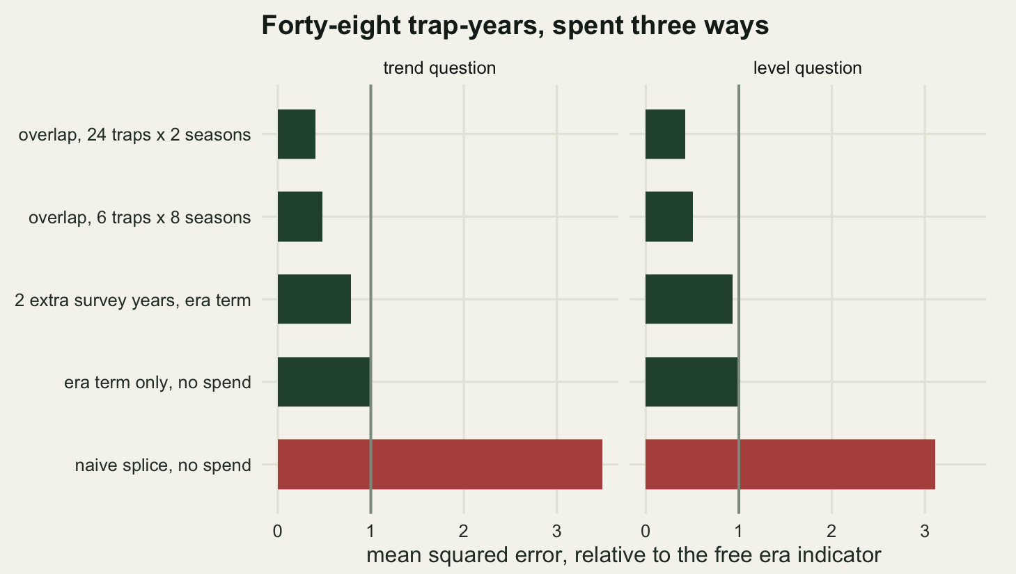
Dual running is not free, and the observer-nights it consumes could have gone somewhere else. The trade between more sites and more years has a closed form for trend monitoring (Gerrodette 1987) and the previous post in that series works it through; a calibration overlap is a third axis, and it is not in the formula. Fix the budget at 48 extra trap-years, which is two extra seasons of the whole network, and put three uses of it side by side: the whole network dual-running for two seasons, six traps dual-running for eight, and two extra survey years added to the end of the series with an era indicator and no trial at all. The two free options stay in the table for scale.
n_rep2 <- 2000
opt <- matrix(NA_real_, n_rep2, 10)
for (b in seq_len(n_rep2)) {
  z <- sim_net(740000 + b)
  tru_lv <- beta_true * (t_c[n_year] - t_c[1]) + z$u_t[n_year] - z$u_t[1]
  obs_lv <- z$idx[n_year] - z$idx[1]
  d_wide <- conv_est(z, seq_len(n_trap), budget %/% n_trap)
  d_deep <- conv_est(z, seq_len(6), budget %/% 6)
  m_short <- lm(z$idx ~ t_c + new_era)
  m_long <- lm(z$idx_long ~ t_l + era_l)
  opt[b, ] <- c(tr_slope(z$idx - d_wide * new_era),
                tr_slope(z$idx - d_deep * new_era),
                unname(coef(m_long)[2]), unname(coef(m_short)[2]),
                tr_slope(z$idx),
                obs_lv - d_wide - tru_lv, obs_lv - d_deep - tru_lv,
                obs_lv - unname(coef(m_long)[3]) - tru_lv,
                obs_lv - unname(coef(m_short)[3]) - tru_lv,
                obs_lv - tru_lv)
}

opt_lab <- c("overlap, 24 traps x 2 seasons", "overlap, 6 traps x 8 seasons",
             "2 extra survey years, era term", "era term only, no spend",
             "naive splice, no spend")
budget_tab <- data.frame(
  option = opt_lab,
  spend = c(budget, budget, budget, 0, 0),
  trend_bias_dec = 10 * (colMeans(opt[, 1:5]) - beta_true),
  trend_rmse_dec = 10 * sqrt(colMeans((opt[, 1:5] - beta_true)^2)),
  level_rmse = sqrt(colMeans(opt[, 6:10]^2)))
budget_tab$trend_mse_rel <-
  (budget_tab$trend_rmse_dec / budget_tab$trend_rmse_dec[4])^2
budget_tab$level_mse_rel <-
  (budget_tab$level_rmse / budget_tab$level_rmse[4])^2
print(budget_tab, digits = 4, row.names = FALSE)
option spend trend_bias_dec trend_rmse_dec level_rmse
overlap, 24 traps x 2 seasons 48 1.439e-03 0.07146 0.1476
overlap, 6 traps x 8 seasons 48 -1.161e-03 0.07719 0.1603
2 extra survey years, era term 48 -2.212e-03 0.09925 0.2183
era term only, no spend 0 -4.617e-05 0.11184 0.2261
naive splice, no spend 0 -2.003e-01 0.20887 0.3988
trend_mse_rel level_mse_rel
0.4082 0.4265
0.4763 0.5030
0.7875 0.9324
1.0000 1.0000
3.4880 3.1116Against the free era indicator, 48 trap-years of dual running across the whole network cut the trend mean squared error to 0.408 of it, and the same 48 trap-years bought as two extra survey years cut it only to 0.788. For a scheme facing a method change, the calibration is the better buy, and it is not close. The reason is in the exchange rate again: two extra years at the end lengthen the series and dilute a step by a little, but they leave the conversion exactly as unknown as it was, whereas the trial attacks the term that dominates.
One prediction did not come out. Going in, the expectation was an asymmetry: that a calibration buys the level and the era indicator handles the trend, so that the two options would separate sharply depending on the question. They do not. The whole-network trial takes the trend mean squared error to 0.408 of the era indicator’s and the level mean squared error to 0.427, which is the same factor to within Monte Carlo noise, and the six-trap trial gives 0.476 and 0.503. The reason is visible once stated: both questions are damaged by the same quantity, the error in the conversion, and both are damaged in proportion to it. The trend pays 0.5364 per decade per unit of conversion error, the level pays one unit per unit, and relative to the precision each question already had those two prices happen to be close. The genuine asymmetry is elsewhere in the table: the naive splice is 3.488 times worse than the era indicator for the trend and 3.112 times for the level, and it is the only option in the table that is biased rather than merely imprecise.
Buying survey years is a poor third for a different reason at the level question. Two extra years take the level mean squared error only to 0.932 of the era indicator’s, which is nothing at all: extra years at the end of a series barely improve an era term whose problem is its collinearity with time, not its sample size.
Where the trial runs matters more than how long it runs
Two trials of the same total size can be laid out differently: a few traps for many seasons, or many traps for a few. The total number of dual trap-years is held at 48 and the shape is varied.
shape <- data.frame(traps = c(4, 6, 8, 12, 24), years = c(12, 8, 6, 4, 2))
n_rep3 <- 2000
sh_out <- matrix(NA_real_, nrow(shape), 3)
for (r in seq_len(nrow(shape))) {
  dv <- tvals <- numeric(n_rep3)
  for (b in seq_len(n_rep3)) {
    z <- sim_net(750000 + b)
    dh <- conv_est(z, seq_len(shape$traps[r]), shape$years[r])
    dv[b] <- dh - z$d_star
    tvals[b] <- tr_slope(z$idx - dh * new_era)
  }
  sh_out[r, ] <- c(mean(dv), sd(dv), rmse_dec(tvals))
}
shape$conv_bias <- sh_out[, 1]
shape$conv_sd <- sh_out[, 2]
shape$trend_rmse_dec <- sh_out[, 3]
print(round(shape, 5))
traps years conv_bias conv_sd trend_rmse_dec
1 4 12 0.01117 0.10550 0.07861
2 6 8 0.00598 0.09987 0.07691
3 8 6 0.00297 0.09547 0.07457
4 12 4 0.00083 0.08933 0.07222
5 24 2 -0.00148 0.08386 0.07045Spreading the trial thinly is better, and by less than the section heading promises. Four traps for twelve seasons gives a trend error of 7.56 per cent per decade and the whole network for two seasons gives 6.8, a difference of 24.5 per cent in mean squared error. The mechanism is the between-trap part of the conversion variance, which no number of seasons at four traps can reduce, and at this level of trap-to-trap variation that floor is a modest part of the total. The practical reading is that a scheme with an awkward field constraint, two observers willing to run two lamps for a decade, is not throwing its money away.
What does matter is which traps. A trial has to go somewhere, and the sites it goes to are rarely drawn at random: they are the ones with keen operators, easy access and catches big enough to compare, which in this network means the richest traps, which are exactly the ones whose conversion is furthest from the network average. The estimator matters too. Averaging the per-night log ratios answers a different question from taking the ratio of the two totals, because the network index is built from totals.
conv_mlog <- function(z, traps, k) {
  cc <- (ov_max - k + 1):ov_max
  mean(log((z$new_ov[traps, cc, drop = FALSE] + 0.5) /
             (z$old_ov[traps, cc, drop = FALSE] + 0.5)))
}

n_rep4 <- 2000
pick <- matrix(NA_real_, n_rep4, 6)
for (b in seq_len(n_rep4)) {
  z <- sim_net(760000 + b)
  top <- order(z$a_i, decreasing = TRUE)[seq_len(6)]
  d_rand <- conv_est(z, seq_len(6), 8)
  d_top <- conv_est(z, top, 8)
  d_ml <- conv_mlog(z, seq_len(6), 8)
  pick[b, ] <- c(d_rand - z$d_star, d_top - z$d_star, d_ml - z$d_star,
                 tr_slope(z$idx - d_rand * new_era),
                 tr_slope(z$idx - d_top * new_era),
                 tr_slope(z$idx - d_ml * new_era))
}
pick_tab <- data.frame(
  overlap = c("six traps at random", "the six biggest catches",
              "six at random, mean of log ratios"),
  conv_bias = colMeans(pick[, 1:3]),
  conv_rmse = sqrt(colMeans(pick[, 1:3]^2)),
  trend_bias_dec = 10 * (colMeans(pick[, 4:6]) - beta_true),
  trend_rmse_dec = 10 * sqrt(colMeans((pick[, 4:6] - beta_true)^2)))
print(pick_tab, digits = 4, row.names = FALSE)
overlap conv_bias conv_rmse trend_bias_dec
six traps at random 0.008659 0.09745 -0.00502
the six biggest catches -0.125718 0.15055 0.06706
six at random, mean of log ratios 0.051685 0.10470 -0.02810
trend_rmse_dec
0.07559
0.09609
0.07874Eight seasons at six traps chosen at random recovers the conversion with a bias of 0.0087 and leaves the trend with a bias of -0.005 per decade. The same eight seasons at the six biggest catches recovers a conversion 0.1257 too low, which is 33.4 per cent of the whole step, and turns the trend bias into 0.0671 per decade: the sign has flipped, and a declining population is now being read as declining less. The trend error rises from 7.28 to 9.16 per cent per decade. Averaging log ratios instead of taking the ratio of totals is a smaller version of the same mistake in the opposite direction: it targets the unweighted mean conversion rather than the catch-weighted one, biasing the conversion by 0.0517 and the trend by -0.0281 per decade, with the trial itself perfectly well run.
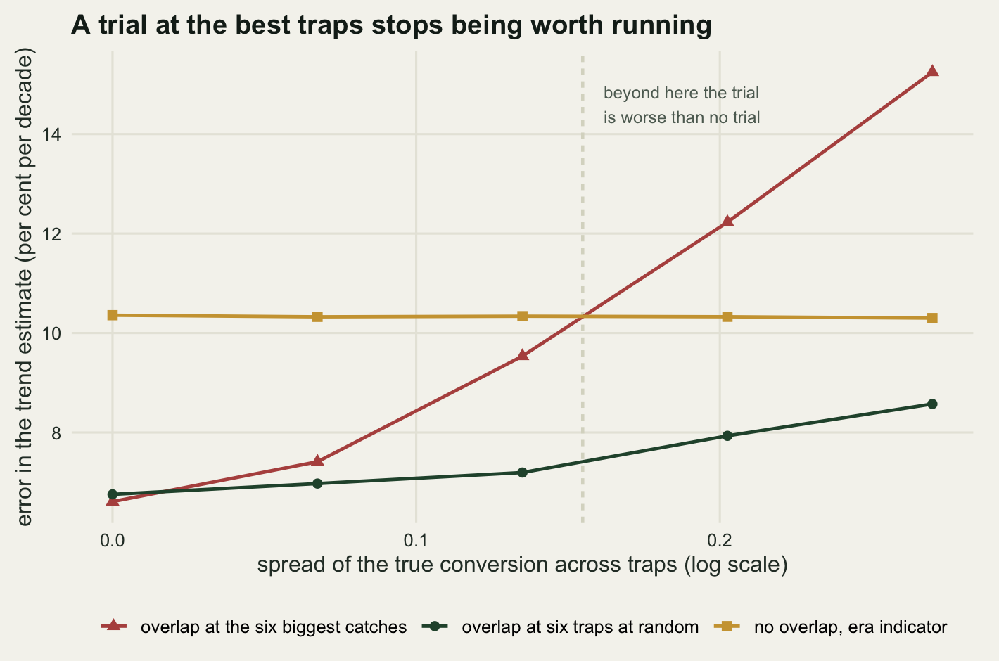
How far can the trap selection go before the trial is a liability? That depends on how much the conversion actually varies from trap to trap, which is a fact about the two lamps rather than about the design, so it is worth sweeping.
gam_grid <- c(0, -0.15, -0.3, -0.45, -0.6)
n_rep5 <- 800
gam_tab <- t(vapply(gam_grid, function(g) {
  vt <- vr <- ve <- numeric(n_rep5)
  for (b in seq_len(n_rep5)) {
    z <- sim_net(770000 + b, gam = g)
    top <- order(z$a_i, decreasing = TRUE)[seq_len(6)]
    vt[b] <- tr_slope(z$idx - conv_est(z, top, 8) * new_era)
    vr[b] <- tr_slope(z$idx - conv_est(z, seq_len(6), 8) * new_era)
    ve[b] <- unname(coef(lm(z$idx ~ t_c + new_era))[2])
  }
  c(conv_sd_across_traps = abs(g) * sd_trap, top_rmse_dec = rmse_dec(vt),
    rand_rmse_dec = rmse_dec(vr), era_rmse_dec = rmse_dec(ve))
}, numeric(4)))
print(round(gam_tab, 5))
conv_sd_across_traps top_rmse_dec rand_rmse_dec era_rmse_dec
[1,] 0.0000 0.06838 0.06995 0.10935
[2,] 0.0675 0.07701 0.07228 0.10899
[3,] 0.1350 0.10021 0.07467 0.10913
[4,] 0.2025 0.13044 0.08265 0.10900
[5,] 0.2700 0.16543 0.08963 0.10870cross <- approx(gam_tab[, "top_rmse_dec"] - gam_tab[, "era_rmse_dec"],
gam_tab[, "conv_sd_across_traps"], xout = 0)$y
print(round(c(crossover_conversion_sd = cross,
this_post_conversion_sd = abs(gam_c) * sd_trap), 4))crossover_conversion_sd this_post_conversion_sd
0.1548 0.1350 The crossing is at a conversion spread of 0.1548 on the log scale across traps. Below that, a trial at the six best traps is still better than no trial; above it, eight seasons of fieldwork produce an answer worse than a dummy variable. The network in this post sits at 0.135, just under the line, which is the uncomfortable place to be: the trial is worth running, but only just, and nothing in its output would tell the scheme how close to the line it was. The trial at six random traps stays clear of the era indicator across the whole sweep, so the fix is in the sampling of traps rather than in the length of the trial.
A calibration is an estimate, and the interval has to say so
Once the conversion is subtracted, the corrected series goes into lm() like any other series, and the standard error that comes back is the standard error of a regression on data treated as given. It knows nothing about where the correction came from. The fix is the delta method: the trend is a function of the index and of the conversion estimate, its derivative with respect to the conversion is minus the exchange rate, and the two variances add.
\[\operatorname{Var}(\hat\beta) \;\approx\; \operatorname{Var}_{\text{lm}}(\hat\beta) \;+\; \left(\frac{6k(n-k)}{n(n^2-1)}\right)^{2} \operatorname{Var}(\hat\delta)\]
The remaining question is where \(\operatorname{Var}(\hat\delta)\) comes from, and the honest answer is not the within-trap noise, because the trap-to-trap variation in the conversion is part of the error too. A jackknife over traps carries both.
jack_var <- function(z, traps, k) {
  m <- length(traps)
  ps <- vapply(seq_len(m), function(j) conv_est(z, traps[-j], k), numeric(1))
  (m - 1) / m * sum((ps - mean(ps))^2)
}

n_rep6 <- 2000
prop <- matrix(NA_real_, n_rep6, 6)
tq <- qt(0.975, n_year - 2)
for (b in seq_len(n_rep6)) {
  z <- sim_net(780000 + b)
  dh <- conv_est(z, seq_len(6), 5)
  m <- lm((z$idx - dh * new_era) ~ t_c)
  se_lm <- summary(m)$coefficients[2, 2]
  vj <- jack_var(z, seq_len(6), 5)
  se_pr <- sqrt(se_lm^2 + xr_yr^2 * vj)
  bh <- unname(coef(m)[2])
  prop[b, ] <- c(bh, se_lm, se_pr, sqrt(vj),
                 abs(bh - beta_true) < tq * se_lm,
                 abs(bh - beta_true) < tq * se_pr)
}
print(round(c(true_sd_dec = 10 * sd(prop[, 1]),
              reported_se_dec = 10 * mean(prop[, 2]),
              propagated_se_dec = 10 * mean(prop[, 3]),
              understatement = sd(prop[, 1]) / mean(prop[, 2]),
              jackknife_conv_sd = mean(prop[, 4]),
              true_conv_sd = sd(sw_dd[, ov_len == 5])), 4))
true_sd_dec reported_se_dec propagated_se_dec understatement
0.0810 0.0548 0.0840 1.4781
jackknife_conv_sd true_conv_sd
0.1143 0.1183 print(round(c(coverage_as_reported = mean(prop[, 5]),
coverage_propagated = mean(prop[, 6]), nominal = 0.95), 4))coverage_as_reported coverage_propagated nominal
0.8310 0.9515 0.9500 With a five-season trial at six traps, the spread of the trend estimate across networks is 0.081 per decade and the standard error the regression reports is 0.0548. The reported figure understates the real one by a factor of 1.478, and the interval built on it covers the true trend 83.1 per cent of the time instead of ninety-five. Adding the jackknife term takes the average standard error to 0.084 per decade and coverage to 95.15 per cent. The jackknife itself is honest about the conversion: it returns 0.1143 against a true spread of 0.1183, from six traps.
That understatement is worth holding next to the earlier result. A trial of this size takes the trend error below the era indicator’s, but a scheme that then reports the uncorrected interval is claiming a precision it has not got, and the amount it is overclaiming, 47.8 per cent on the standard error, is larger than the 25.6 per cent by which the trial cut the real error below the era indicator’s. Bland and Altman (1986) made the same point about clinical method comparison: the agreement between two methods is itself estimated, with limits, and quoting the conversion without them is where the trouble starts.
The limit: one number, two quantities
Everything so far assumed that the two lamps measure the same thing up to a constant. Suppose they do not. The annual figure is the catch of what the recording card calls one species, and suppose it is really two forms with different sizes and different flight periods: group A, which is stable and which both lamps take alike, and group B, which is declining fast and which the actinic tube takes much less well.
w_b <- 0.30
b_a <- 0
b_b <- -0.05
rho <- 0.35
eff_a <- f_meth / ((1 - w_b) + rho * w_b)
grp_b <- function(tt) w_b * exp(b_b * tt)
tot_old <- function(tt) (1 - w_b) * exp(b_a * tt) + grp_b(tt)
tot_new <- function(tt) eff_a * ((1 - w_b) * exp(b_a * tt) + rho * grp_b(tt))
true_mix <- unname(coef(lm(log(tot_old(t_c)) ~ t_c))[2])
conv_curve <- log(tot_new(t_c) / tot_old(t_c))

mix_tab <- t(vapply(1:12, function(kk) {
  cc <- (k_old - kk + 1):k_old
  d_k <- log(sum(tot_new(t_c[cc])) / sum(tot_old(t_c[cc])))
  ser <- log(tot_old(t_c)) * (1 - new_era) +
    (log(tot_new(t_c)) - d_k) * new_era
  sl <- unname(coef(lm(ser ~ t_c))[2])
  c(overlap_years = kk, conversion_used = d_k, recovered_dec = 10 * sl,
    truth_dec = 10 * true_mix, shortfall_pct = 100 * (1 - sl / true_mix))
}, numeric(5)))
print(round(mix_tab, 5))
overlap_years conversion_used recovered_dec truth_dec shortfall_pct
[1,] 1 -0.33277 -0.11351 -0.152 25.32452
[2,] 2 -0.33716 -0.11115 -0.152 26.87167
[3,] 3 -0.34164 -0.10875 -0.152 28.45363
[4,] 4 -0.34622 -0.10629 -0.152 30.07089
[5,] 5 -0.35091 -0.10378 -0.152 31.72395
[6,] 6 -0.35569 -0.10121 -0.152 33.41327
[7,] 7 -0.36059 -0.09859 -0.152 35.13929
[8,] 8 -0.36558 -0.09591 -0.152 36.90244
[9,] 9 -0.37068 -0.09317 -0.152 38.70312
[10,] 10 -0.37589 -0.09038 -0.152 40.54170
[11,] 11 -0.38121 -0.08752 -0.152 42.41852
[12,] 12 -0.38664 -0.08461 -0.152 44.33390print(round(c(share_b_first = grp_b(t_c[1]) / tot_old(t_c[1]),
share_b_last = grp_b(t_c[n_year]) / tot_old(t_c[n_year]),
conv_first = conv_curve[1], conv_swap = conv_curve[k_old],
conv_last = conv_curve[n_year],
efficiency_group_a = eff_a, efficiency_group_b = eff_a * rho), 4)) share_b_first share_b_last conv_first conv_swap
0.4570 0.1791 -0.4641 -0.3328
conv_last efficiency_group_a efficiency_group_b
-0.2354 0.8944 0.3130 Group B is 30 per cent of the catch at the midpoint of the series, the new lamp takes group A at 0.8944 of the old lamp’s rate and group B at 0.313, and the two together happen to give the same overall factor of 0.72 at the midpoint that the rest of the post used. So a trial run at the changeover would report a familiar number, and it would still be the wrong kind of number.
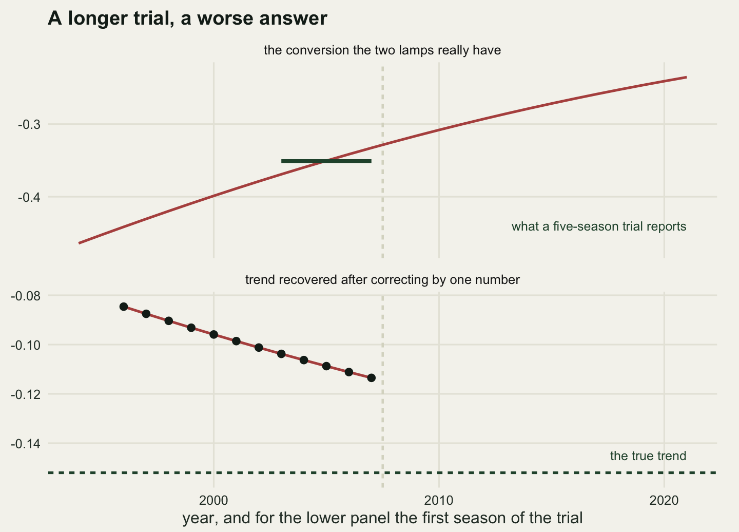
There is no constant to estimate. The conversion is -0.4641 in the first year of the series, -0.3328 in the year of the changeover and -0.2354 in the last, because group B’s share of the catch falls from 45.7 per cent to 17.9 per cent while the trial reports one number. Correcting by that number recovers a trend of -0.1135 per decade from a single-season trial against a truth of -0.152, a shortfall of 25.3 per cent of the real decline. A twelve-season trial recovers -0.0846, a shortfall of 44.3 per cent. The longer trial is further from the truth, because a longer trial reaches back into earlier seasons when group B was commoner and the conversion was steeper, so the one number it reports is a better estimate of a period the scheme does not care about.
ser_raw <- log(tot_old(t_c)) * (1 - new_era) + log(tot_new(t_c)) * new_era
era_mix <- 10 * unname(coef(lm(ser_raw ~ t_c + new_era))[2])
ser_cls <- log(tot_old(t_c)) * (1 - new_era) +
  log((1 - w_b) * exp(b_a * t_c) + grp_b(t_c)) * new_era
cls_mix <- 10 * unname(coef(lm(ser_cls ~ t_c))[2])
print(round(c(truth_dec = 10 * true_mix, era_term_dec = era_mix,
              one_season_trial_dec = mix_tab[1, "recovered_dec"],
              per_class_conversion_dec = cls_mix), 5))
truth_dec era_term_dec
-0.15200 -0.11883
one_season_trial_dec.recovered_dec per_class_conversion_dec
-0.11351 -0.15200 ov5 <- (k_old - 4):k_old
df_dr <- 6 * length(ov5) - 2
dr_slope <- unname(coef(lm(conv_curve[ov5] ~ I(t_c[ov5])))[2])
se_dr <- sqrt(2 * sd_ty^2 + 2 / exp(mu_log)) /
sqrt(6 * sum((t_c[ov5] - mean(t_c[ov5]))^2))
pw_dr <- 1 - pt(qt(0.975, df_dr), df_dr, dr_slope / se_dr) +
pt(-qt(0.975, df_dr), df_dr, dr_slope / se_dr)
print(round(c(drift_within_5_seasons = conv_curve[k_old] - conv_curve[k_old - 4],
drift_after_the_swap = conv_curve[n_year] - conv_curve[k_old],
drift_slope_per_year = dr_slope, se_of_that_slope = se_dr,
power_to_detect_drift = pw_dr), 5))drift_within_5_seasons drift_after_the_swap drift_slope_per_year
0.03632 0.09740 0.00908
se_of_that_slope power_to_detect_drift
0.06811 0.05190 The trial cannot see this from inside itself. Across the five seasons of a five-season overlap the true conversion moves by 0.0363, against 0.0974 across the years that follow the changeover. A regression of the trial’s log ratio on year within the trial has a true slope of 0.00908 per year and a standard error of 0.0681, so the test for a drifting conversion has power 0.0519, which is its own false-positive rate. The trial reports a tight conversion, a flat log ratio and no warning of any kind, and it is measuring something the scheme did not ask about.
Nothing statistical repairs this. The era indicator is not a fix either: it returns -0.1188 per decade against the truth of -0.152, less wrong than the long trial and wrong all the same, because after the changeover the network is simply counting a different thing. What does repair it is a field decision taken at the same time as the trial. If the trial’s catch is identified and counted at the level at which the two methods could plausibly differ, by species, by size class, by night of the flight period, then a conversion can be estimated for each class and applied separately. The same overlap data, sorted, recovers -0.152 per decade, which is the truth exactly, because correcting each class by its own factor reconstructs the old-lamp total rather than approximating it. Sorting the trial catch costs bench time in the winter and nothing in the field, and it is the difference between a calibration that is about the index and one that is about a number.
The general form of the rule is that a trial must record what the two methods disagree about, not just how much they disagree in total. Double sampling in bird surveys has the same structure: a cheap method is calibrated against an intensive one on a subset, and the calibration is only transportable to the extent that the ratio between them is stable across the conditions it will be applied to (Bart and Earnst 2002). A ratio measured on last decade’s community and applied to this decade’s is a transport that nobody checked.
What to take away
A scheme planning a method change has three options, and the free one is better than most people expect. An era indicator costs a degree of freedom and no fieldwork, and it takes the trend error from 18.89 per cent per decade to 10.72. That is the number a trial has to beat, and a trial of one season at six traps does not beat it. Two seasons at six traps, 12 dual trap-years, is where the calibration starts paying, and season 3 is the last one that buys a full percentage point per decade. After that the price climbs: by the twelfth season a point costs 10.4 seasons instead of 0.87.
At a matched budget of 48 trap-years the calibration is the better spend, by a wide margin over buying survey years: mean squared error 0.408 of the era indicator’s against 0.788 for two extra years. The asymmetry I went in expecting, that calibration buys the level and the era indicator handles the trend, is not there: the factors are 0.408 and 0.427, near enough the same, because both questions are damaged by the same conversion error in the same proportion. The real division in the table is between the naive splice, which is biased, and everything else, which is not.
Two things about the shape of the trial went the other way from what the design intuition suggested. Concentrating the same effort on four traps rather than twenty-four costs only 24.5 per cent in mean squared error, so the arrangement is a weaker lever than expected. Choosing those traps badly is a much stronger one: eight seasons at the six richest traps biases the conversion by -0.1257 and the trend by 0.0671 per decade towards zero, and once the conversion varies across traps by more than 0.155 on the log scale, that trial is worse than no trial. Neither the length of the trial nor its own output gives any hint of this.
Two smaller results carry further than the moth network. The conversion estimator has to match the index: the ratio of the two totals is right for an index built from totals, and averaging log ratios biases the conversion by 0.0517 here. And the conversion is an estimate, so the trend interval has to carry its variance; the delta method with a jackknife over traps moved coverage from 83.1 to 95.15 per cent, and the correction to the standard error, 47.8 per cent, was larger than the whole gain the trial bought.
The honest limit is that the overlap identifies the conversion only if the two methods track the same quantity up to that conversion. When they do not, a longer trial makes the answer worse rather than better, the trial’s internal check for a drifting conversion has power 0.052, and the report is a confident number about the wrong thing. There is no statistical repair, and there is a cheap field one: sort and identify the trial’s catch at the level at which the two methods could differ, and estimate a conversion for each class. In the mixture above that recovers -0.152 per decade against a truth of -0.152, from exactly the same nights of fieldwork.
References
Merckx T, Slade EM 2014 Insect Conservation and Diversity 7(5):453-461 (10.1111/icad.12068)
Infusino M, Brehm G, Di Marco C, Scalercio S 2017 European Journal of Entomology 114:25-33 (10.14411/eje.2017.004)
van Grunsven RHA, Donners M, Boekee K, Tichelaar I, van Geffen KG, Groenendijk D, Berendse F, Veenendaal EM 2014 Journal of Insect Conservation 18(2):225-231 (10.1007/s10841-014-9633-9)
Conrad KF, Warren MS, Fox R, Parsons MS, Woiwod IP 2006 Biological Conservation 132(3):279-291 (10.1016/j.biocon.2006.04.020)
Isaac NJB, van Strien AJ, August TA, de Zeeuw MP, Roy DB 2014 Methods in Ecology and Evolution 5(10):1052-1060 (10.1111/2041-210X.12254)
Bart J, Earnst S 2002 The Auk 119(1):36-45 (10.1093/auk/119.1.36)
Bland JM, Altman DG 1986 The Lancet 327(8476):307-310 (10.1016/S0140-6736(86)90837-8)
Gerrodette T 1987 Ecology 68(5):1364-1372 (10.2307/1939220)