library(ggplot2)
library(patchwork)

te_paper  <- "#f5f4ee"
te_ink    <- "#16241d"
te_body   <- "#2c3a31"
te_forest <- "#275139"
te_rust   <- "#b5534e"
te_gold   <- "#c9b458"
te_line   <- "#dad9ca"

theme_datasheet <- function() {
  theme_minimal(base_size = 12) +
    theme(plot.background  = element_rect(fill = te_paper, colour = NA),
          panel.background = element_rect(fill = te_paper, colour = NA),
          panel.grid.major = element_line(colour = te_line, linewidth = 0.3),
          panel.grid.minor = element_blank(),
          text             = element_text(colour = te_body),
          plot.title       = element_text(colour = te_ink, face = "bold"),
          plot.subtitle    = element_text(colour = te_body),
          axis.text        = element_text(colour = te_body),
          strip.text       = element_text(colour = te_ink))
}Reset time and the double-counted hot day
R
temperature
climate
data quality
simulation
ecology tutorial
A min-max thermometer reset in the afternoon counts hot afternoons twice. Simulating time-of-observation bias in R: its size, its cause and its correction.
A field station on the edge of a reserve has kept a min-max thermometer in a Stevenson screen since the 1980s. Whoever is on duty walks out at the end of the working day, writes down the maximum and the minimum, and presses the reset button. Twenty-five years later a student digitises the notebooks into a table with one row per date, a tmax column and a tmin column, and fits a growth model with degree days. A second site in the same study has an iButton logger that is downloaded on the monthly visit and summarised by a script into “days” that run from one download hour to the next. Nothing in either table says at what hour the day ended.
That hour matters. A thermometer reset at 17:00 starts the next reading day at the temperature of 17:00, which on a hot afternoon is close to the day’s maximum. If the following day is cooler, its recorded maximum is not its own afternoon peak but the warm late afternoon of the day before, carried over by the reset. The hot afternoon is counted twice, and nothing in the notebook shows it. Climatologists know this as the time-of-observation bias: Baker (1975) measured it from three years of hourly records at St. Paul, Minnesota, and noted the effect on degree days; Karl and colleagues (1986) built an empirical model of it from hourly records at 79 United States stations; Vose and colleagues (2003) tested the adjustment built on that model and found that it held up, with low residual errors; and it remains one of the adjustments applied to the United States Historical Climatology Network (Menne and colleagues 2009). This post is a demonstration of that known result in the form an ecologist meets it, not a new finding.
The site has several posts that start where this one ends. Degree days and thermal time in R says that what arrives in a spreadsheet is a daily minimum and a daily maximum, and takes the pair as given. Records as a test for trend opens with a station that logs the highest daily maximum temperature of each summer. Splicing a monitoring series prices a method change once its step is known. Dates and times in ecological data treats a clock reading as a time-zone problem. Here the question is one step earlier: how the reset hour manufactures the daily extremes, how large the error is, which part of the simulation produces it, and what a correction borrowed from somewhere else can and cannot repair.
A temperature record with a known calendar day
The simulated station has a temperature value every 10 minutes for 20 years of 365 days. Four pieces add up. A seasonal cycle has a mean of 10 C and swings 10 C either side, coldest in mid January. A synoptic anomaly, the day-to-day weather, is an AR(1) series with coefficient 0.7 and a marginal standard deviation that is one of the design factors; it is drawn once per day and interpolated linearly through the day, so a cold front can arrive at any hour. A diurnal cycle has its minimum at 06:00 and its maximum at 15:00, rising along half a cosine for nine hours and falling along half a cosine for fifteen. Its daily range has a median of 10 C and, at the main station and in half of the later grid, day-to-day variation drawn from a lognormal with log standard deviation 0.25, also interpolated through the day. Last, a small short-term fluctuation with standard deviation 0.3 C and an autocorrelation time of one hour stands for gusts, passing cloud and the thermometer itself. All of these constants were fixed before the first run.
The calendar-day maximum and minimum over the 144 values from 00:00 to 23:50 are the truth. A min-max thermometer reset at hour h reports, for the day on which it is read, the extremes of every value from hour h of the previous day up to and including hour h of that day. The reading at the reset instant belongs to both windows. With 10-minute values that shared value is one of 145, and a later section checks how little it contributes on its own.
steps_day <- 144                       # 10-minute values per day
n_years   <- 20
n_days    <- 365 * n_years
hour_min  <- 6                         # diurnal minimum
hour_max  <- 15                        # diurnal maximum
ar_coef   <- 0.7                       # day-to-day persistence of the weather
range_med <- 10                        # median diurnal range, C
main_syn  <- 2.5                       # synoptic SD at the main station, C
main_amp  <- 0.25                      # log SD of the daily range
main_noise <- 0.3                      # short-term fluctuation SD, C
hot_q     <- 0.9                       # hot day: above the calendar 90th percentile
dd_base   <- 10                        # degree-day base, C

diurnal_shape <- function(hr) {
  out <- numeric(length(hr))
  rising <- hr >= hour_min & hr < hour_max
  out[rising] <- -0.5 * cos(pi * (hr[rising] - hour_min) / (hour_max - hour_min))
  since_peak <- (hr[!rising] - hour_max) %% 24
  out[!rising] <- 0.5 * cos(pi * since_peak / (24 - hour_max + hour_min))
  out
}

make_weather <- function(syn_sd, n = n_days) {
  burn <- 50
  shocks <- rnorm(n + burn, 0, syn_sd * sqrt(1 - ar_coef^2))
  as.numeric(stats::filter(shocks, ar_coef, method = "recursive"))[-seq_len(burn)]
}

make_station <- function(weather, amp_sdlog = main_amp, noise_sd = main_noise,
                         steps = steps_day, iid_noise = FALSE) {
  nd <- length(weather)
  tt <- (seq_len(nd * steps) - 1) / steps
  hr <- (tt %% 1) * 24
  day_mid <- seq_len(nd) - 0.5
  daily_range <- approx(day_mid, range_med * exp(rnorm(nd, 0, amp_sdlog)), tt, rule = 2)$y
  anomaly <- approx(day_mid, weather, tt, rule = 2)$y
  phi_fast <- exp(-(24 / steps))
  fast <- if (noise_sd == 0) 0 else if (iid_noise) rnorm(length(tt), 0, noise_sd) else
    as.numeric(stats::filter(rnorm(length(tt), 0, noise_sd * sqrt(1 - phi_fast^2)),
                             phi_fast, method = "recursive"))
  list(temp = 10 - 10 * cos(2 * pi * ((tt %% 365) - 15) / 365) + anomaly +
         daily_range * diurnal_shape(hr) + fast,
       steps = steps)
}

# window = "closed": from hour h yesterday to hour h today, both included
# "open_end": the reading at hour h today left out; "open_start": the one yesterday left out
reset_extremes <- function(stn, h, window = "closed") {
  v <- stn$temp; s <- stn$steps; nd <- length(v) / s
  cal <- matrix(v, nrow = s)
  off <- h * s / 24
  first <- off + 1 + (window == "open_start")
  blocks <- matrix(v[first:(first + (nd - 1) * s - 1)], nrow = s)
  obs_max <- apply(blocks, 2, max); obs_min <- apply(blocks, 2, min)
  if (window == "closed") {
    end_val <- v[seq(off + 1 + s, by = s, length.out = nd - 1)]
    obs_max <- pmax(obs_max, end_val); obs_min <- pmin(obs_min, end_val)
  }
  list(cal_max = apply(cal, 2, max), cal_min = apply(cal, 2, min),
       obs_max = obs_max, obs_min = obs_min, day = 2:nd)
}

summarise_reset <- function(ext) {
  d <- ext$day
  err_max <- ext$obs_max - ext$cal_max[d]
  err_min <- ext$obs_min - ext$cal_min[d]
  yr <- (d - 1) %/% 365
  hot_thr <- quantile(ext$cal_max, hot_q, names = FALSE)
  c(tmax = mean(err_max), tmin = mean(err_min),
    se_tmax = sd(tapply(err_max, yr, mean)) / sqrt(n_years),
    se_tmin = sd(tapply(err_min, yr, mean)) / sqrt(n_years),
    hot_ratio = sum(ext$obs_max > hot_thr) / sum(ext$cal_max[d] > hot_thr),
    frost_ratio = sum(ext$obs_min < 0) / sum(ext$cal_min[d] < 0),
    share_up = mean(err_max > 0.05))
}
The Monte Carlo standard error of a mean bias comes from the spread of the 20 yearly means. Consecutive years share a little weather through the AR(1) series, but with a coefficient of 0.7 per day the dependence is gone within a fortnight, so the years are treated as independent replicates.
A hot afternoon read twice
set.seed(1709)
weather_main <- make_weather(main_syn)
station_main <- make_station(weather_main)
ext17 <- reset_extremes(station_main, 17)
err17 <- ext17$obs_max - ext17$cal_max[ext17$day]

# illustration: the first day after day 172 (midsummer) whose 17:00 maximum is 3 C too high
show_day <- ext17$day[which(ext17$day > 172 & err17 > 3)[1]]
show_span <- (show_day - 3):(show_day + 2)
trace_idx <- unlist(lapply(show_span, function(k) (k - 1) * steps_day + seq_len(steps_day)))
trace_df <- data.frame(time = (trace_idx - 1) / steps_day,
                       temp = station_main$temp[trace_idx])
day_pts <- data.frame(day = show_span,
                      calendar = ext17$cal_max[show_span],
                      reset_17 = ext17$obs_max[show_span - 1])
day_long <- rbind(data.frame(time = day_pts$day - 1 + hour_max / 24, temp = day_pts$calendar,
                             kind = "calendar-day maximum"),
                  data.frame(time = day_pts$day - 1 + 17 / 24, temp = day_pts$reset_17,
                             kind = "17:00 reading"))
carry_val <- day_pts$reset_17[day_pts$day == show_day]
own_val <- day_pts$calendar[day_pts$day == show_day]
Take the main station, with synoptic standard deviation 2.5 C, and a reset at 17:00. The first day after midsummer (day 172) on which the recorded maximum is more than 3 C above the calendar maximum is day 275 of the series, in early autumn. Its own afternoon peaked at 18.9 C. The notebook says 22.2 C, a value from half past five on the previous, warmer day, just after that day’s 17:00 reset. Over all 7299 days, the recorded maximum is more than 0.05 C above the calendar value on a share of 0.371 of them, and the largest single excess is 6.6 C. The error is almost always zero or positive, because the reading window contains the calendar day’s afternoon and sometimes adds a hotter evening from the day before. It is negative only when the calendar day’s maximum falls after 17:00, as when warm air arrives in the evening: that happens by more than 0.05 C on a share of 0.010 of days, and the largest shortfall is 0.50 C.
ggplot(trace_df, aes(time, temp)) +
  geom_vline(xintercept = show_span - 1 + 17 / 24, colour = te_line, linetype = "dotted",
             linewidth = 0.6) +
  geom_line(colour = te_body, linewidth = 0.5) +
  geom_point(data = day_long, aes(colour = kind, shape = kind), size = 3) +
  scale_colour_manual(values = c("calendar-day maximum" = te_forest, "17:00 reading" = te_rust),
                      name = NULL) +
  scale_shape_manual(values = c("calendar-day maximum" = 16, "17:00 reading" = 17), name = NULL) +
  scale_x_continuous(breaks = show_span - 1, labels = paste("day", show_span)) +
  labs(x = NULL, y = "temperature (C)",
       title = "The warm evening after a reset becomes tomorrow's maximum",
       subtitle = "main station: synoptic SD 2.5 C, 10-minute values") +
  theme_datasheet() +
  theme(legend.position = "top")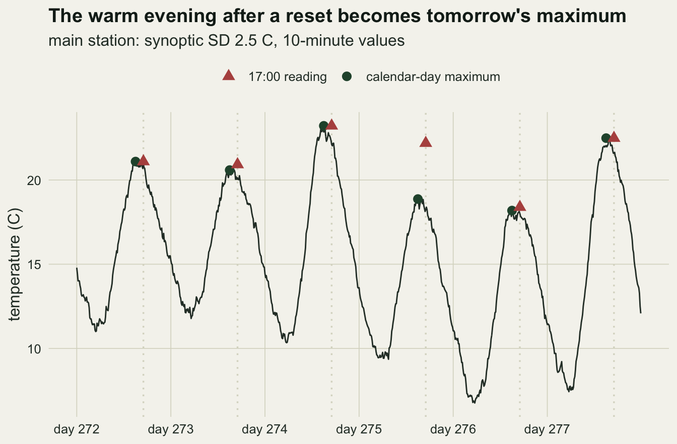
Every reset hour has its own bias
sweep_tab <- do.call(rbind, lapply(0:23, function(h) {
  s <- summarise_reset(reset_extremes(station_main, h))
  data.frame(hour = h, t(s))
}))
sw <- function(h, col) sweep_tab[sweep_tab$hour == h, col]
worst_max_hour <- sweep_tab$hour[which.max(sweep_tab$tmax)]
worst_min_hour <- sweep_tab$hour[which.min(sweep_tab$tmin)]
both_small <- sweep_tab$hour[abs(sweep_tab$tmax) < 0.02 & abs(sweep_tab$tmin) < 0.02]

sweep_long <- rbind(data.frame(hour = sweep_tab$hour, bias = sweep_tab$tmax,
                               se = sweep_tab$se_tmax, extreme = "maximum"),
                    data.frame(hour = sweep_tab$hour, bias = sweep_tab$tmin,
                               se = sweep_tab$se_tmin, extreme = "minimum"))

ext07 <- reset_extremes(station_main, 7)
dd_of <- function(ext, use_obs) {
  d <- ext$day
  if (use_obs) sum(dd_sine(ext$obs_min, ext$obs_max, dd_base))
  else sum(dd_sine(ext$cal_min[d], ext$cal_max[d], dd_base))
}
dd_sine <- function(tn, tx, tb) {
  amp <- (tx - tn) / 2; avg <- (tx + tn) / 2
  out <- pmax(avg - tb, 0)
  st <- tn < tb & tx > tb
  th <- asin(pmin(1, pmax(-1, (tb - avg) / amp)))
  out[st] <- ((1 / pi) * ((avg - tb) * (pi / 2 - th) + amp * cos(th)))[st]
  out
}
dd_true  <- dd_of(ext17, FALSE)
dd_17    <- dd_of(ext17, TRUE)
dd_07    <- dd_of(ext07, TRUE)
dtr_17   <- sw(17, "tmax") - sw(17, "tmin")
dtr_07   <- sw(7, "tmax") - sw(7, "tmin")
Running the same 20 years through a reset at every whole hour gives the bias surface in the next figure. The maximum is inflated for resets from midday to evening, most at 15:00 (+0.80 C), and at 17:00 by +0.52 C with a Monte Carlo standard error of 0.008. Resets at 07:00 and 09:00 leave the maximum alone: -0.001 and -0.001 C. The minimum mirrors this around dawn. A 07:00 reset lowers the mean minimum by 0.49 C, and the worst hour for the minimum is 06:00 at -0.64 C. Moving an afternoon observer to the morning does not remove the bias; it moves it from one column to the other.
The count of hot days moves as well. With a hot day defined as a calendar maximum above the station’s own 90th percentile, the 17:00 record has 1.19 times as many hot days as the calendar, the 15:00 record 1.32 times and the 07:00 record 1.00 times. The morning reset inflates frost days instead, a minimum below 0 C: the 07:00 record has 1.05 times the calendar count. The diurnal range recorded at 17:00 is too wide by 0.52 C and at 07:00 by 0.49 C. Degree days above 10 C by the single sine method, the method of the degree-day post, total 1305 per year from calendar extremes, 1361 from the 17:00 record (+4.3 per cent) and 1268 from the 07:00 record (-2.8 per cent).
In this model the resets at 00:00, 01:00, 10:00, 11:00, 21:00, 22:00, 23:00 bias neither extreme by more than 0.02 C, because they fall well away from both the 06:00 minimum and the 15:00 maximum. That result belongs to the shape assumed here. A station with a later minimum in winter, or with fronts that tend to arrive at a particular hour, would move those quiet hours.
sweep_plot <- ggplot(sweep_long, aes(hour, bias, colour = extreme, fill = extreme)) +
  geom_hline(yintercept = 0, colour = te_ink, linewidth = 0.4) +
  geom_vline(xintercept = c(hour_min, hour_max), colour = te_line, linetype = "dashed",
             linewidth = 0.6) +
  geom_ribbon(aes(ymin = bias - 2 * se, ymax = bias + 2 * se), colour = NA, alpha = 0.25) +
  geom_line(linewidth = 0.9) +
  geom_point(size = 1.8) +
  scale_colour_manual(values = c(maximum = te_rust, minimum = te_forest), name = "recorded") +
  scale_fill_manual(values = c(maximum = te_rust, minimum = te_forest), name = "recorded") +
  scale_x_continuous(breaks = seq(0, 23, by = 3), labels = sprintf("%02d:00", seq(0, 23, by = 3))) +
  labs(x = "reset hour", y = "bias in mean extreme (C)",
       title = "The reset hour decides which extreme is wrong",
       subtitle = "20 years of 10-minute values, synoptic SD 2.5 C") +
  theme_datasheet() +
  theme(legend.position = "top")
sweep_plot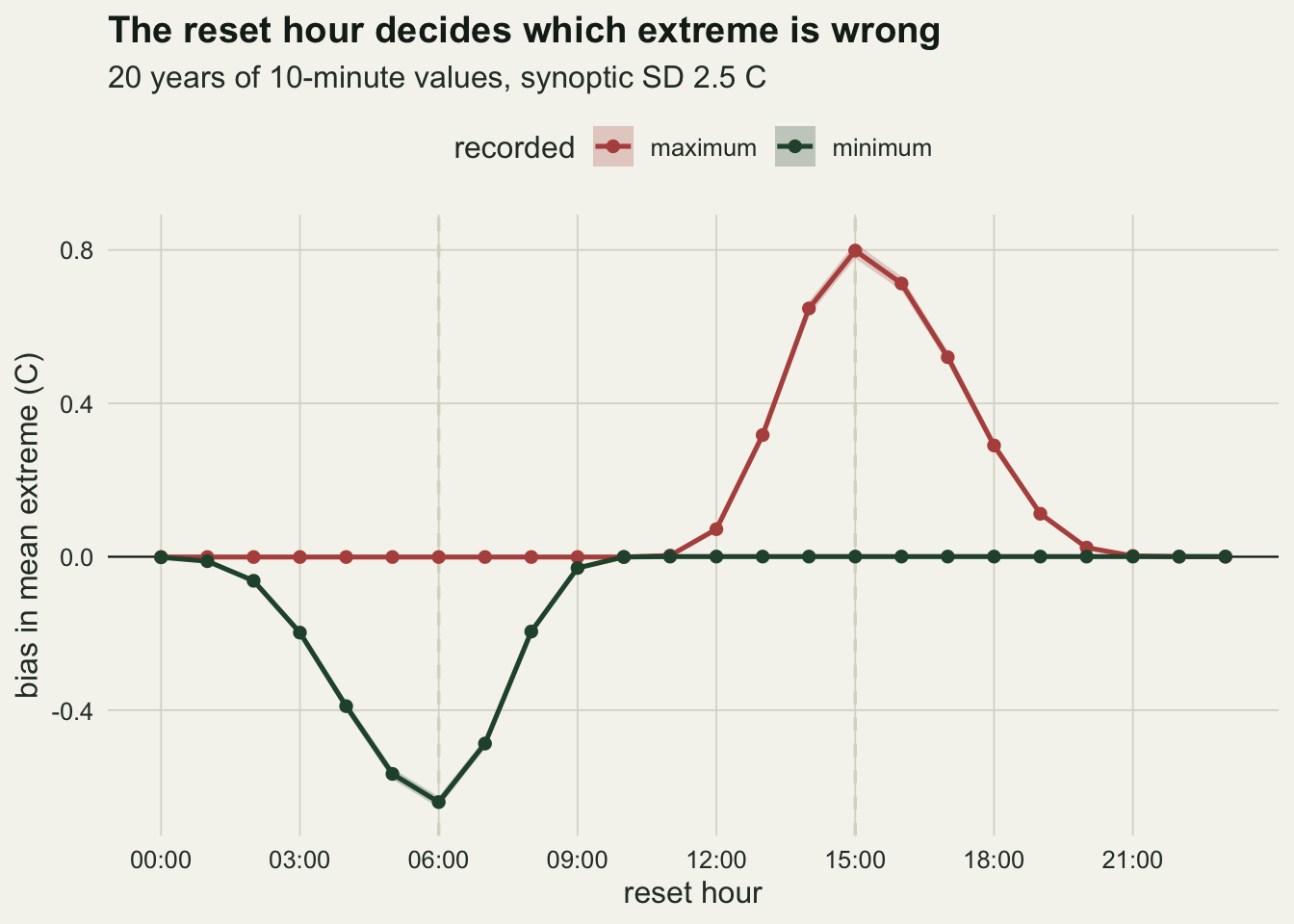
The carried-over reading, not the extra reading
A reviewer’s first question about this set-up is whether the bias comes from counting one reading twice. With hourly values, the window from 17:00 yesterday to 17:00 today holds 25 readings and the calendar day 24, and a maximum over 25 noisy values is larger on average than a maximum over 24 whatever the weather does. That artefact exists, so the simulation has to be run in a form that separates it.
Three window rules pull the pieces apart. The closed window keeps both reset readings. Dropping the reading at the end of the window keeps 24 values and keeps the carry-over from yesterday. Dropping the reading at the start keeps 24 values and removes the one value that carries yesterday’s late afternoon. Each rule is applied to hourly values with independent noise, the form in which the artefact would be largest, to hourly values with the one-hour autocorrelated noise, and to 10-minute values, for a station with no weather at all (synoptic SD 0, no range variation), a station with range variation only, and the main station.
set.seed(2203)
win_cells <- data.frame(station = c("no day-to-day change", "range variation only", "main station"),
                        syn = c(0, 0, main_syn), amp = c(0, main_amp, main_amp))
win_forms <- data.frame(form = c("hourly, independent noise", "hourly, autocorrelated noise",
                                 "10-minute, autocorrelated noise"),
                        steps = c(24, 24, steps_day), iid = c(TRUE, FALSE, FALSE))
# a 2-minute form, run for the main station only, checks the continuous limit
fine_form <- data.frame(form = "2-minute, autocorrelated noise", steps = 720, iid = FALSE)
win_rules <- c("closed", "open_end", "open_start")
win_tab <- do.call(rbind, lapply(seq_len(nrow(win_cells)), function(i) {
  wthr <- make_weather(win_cells$syn[i])
  forms_i <- if (win_cells$station[i] == "main station") rbind(win_forms, fine_form) else win_forms
  do.call(rbind, lapply(seq_len(nrow(forms_i)), function(j) {
    stn <- make_station(wthr, amp_sdlog = win_cells$amp[i], steps = forms_i$steps[j],
                        iid_noise = forms_i$iid[j])
    do.call(rbind, lapply(win_rules, function(r) {
      s <- summarise_reset(reset_extremes(stn, 17, r))
      data.frame(station = win_cells$station[i], form = forms_i$form[j], rule = r,
                 bias = s[["tmax"]], se = s[["se_tmax"]])
    }))
  }))
}))
wt <- function(st, fm, r, col = "bias") {
  win_tab[win_tab$station == st & win_tab$form == fm & win_tab$rule == r, col]
}
h_iid <- "hourly, independent noise"; h_ar <- "hourly, autocorrelated noise"
m10 <- "10-minute, autocorrelated noise"; m2 <- "2-minute, autocorrelated noise"
st0 <- "no day-to-day change"; st_amp <- "range variation only"; st_main <- "main station"
extra_reading <- wt(st0, h_iid, "closed") - wt(st0, h_iid, "open_end")
spread_m10 <- max(tapply(win_tab$bias[win_tab$form == m10], win_tab$station[win_tab$form == m10],
                         function(b) diff(range(b))))
spread_m2 <- diff(range(win_tab$bias[win_tab$form == m2]))
main_m2 <- win_tab$bias[win_tab$form == m2]
win_tab <- win_tab[win_tab$form != m2, ]    # the figure keeps the three forms run at every station
win_tab$rule_lab <- factor(c(closed = "both reset readings", open_end = "end reading dropped",
                             open_start = "start reading dropped")[win_tab$rule],
                           levels = c("both reset readings", "end reading dropped",
                                      "start reading dropped"))
win_tab$station <- factor(win_tab$station, levels = win_cells$station)
win_tab$form <- factor(win_tab$form, levels = win_forms$form)
The pure extra-reading effect is the difference between the closed window and the end-dropped window at the station with no day-to-day change and independent hourly noise: +0.008 C. At that station every rule gives a bias of at most 0.017 C. The carry-over is a different size. With range variation only, the hourly closed window gives +0.28 C, dropping the end reading gives +0.28 C, and dropping the start reading gives +0.11 C. At the main station the three hourly values are +0.54, +0.54 and +0.32 C, and the 10-minute closed window gives +0.51 C.
A 24-reading window, then, is not a single thing. The one that drops the end reading agrees with the closed window. The one that drops the start reading removes the 17:00 value of the previous day, and with hourly values that value stands in for the whole hour from 17:00 to 18:00, when the air is still near its peak. A real thermometer has no such gap: it starts recording the moment it is reset. The 10-minute rows approach the continuous limit without reaching it: the three rules differ there by at most 0.037 C at any station. Run at the main station with 2-minute values, they lie between +0.500 and +0.508 C, against +0.514 C for the closed window at 10 minutes. The headline numbers in this post come from the 10-minute values.
ggplot(win_tab, aes(bias, form, colour = rule_lab, shape = rule_lab)) +
  geom_vline(xintercept = 0, colour = te_ink, linewidth = 0.4) +
  geom_errorbar(aes(xmin = bias - 2 * se, xmax = bias + 2 * se), orientation = "y",
                width = 0.25, position = position_dodge(width = 0.6), linewidth = 0.5) +
  geom_point(size = 2.6, position = position_dodge(width = 0.6)) +
  facet_wrap(~ station, ncol = 3) +
  scale_x_continuous(breaks = c(0, 0.25, 0.5), expand = expansion(mult = c(0.05, 0.12))) +
  scale_colour_manual(values = c(te_rust, te_gold, te_forest), name = NULL) +
  scale_shape_manual(values = c(16, 17, 15), name = NULL) +
  labs(x = "bias in mean maximum (C)", y = NULL,
       title = "Hourly data: dropping the start reading shrinks the bias",
       subtitle = "reset at 17:00; 20 years per cell") +
  theme_datasheet() +
  theme(legend.position = "top", plot.title.position = "plot")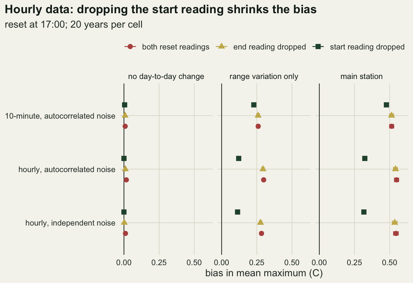
Weather sets the size
set.seed(3119)
grid_tab <- expand.grid(syn = c(0, 0.5, 1.5, 2.5, 3.5), amp = c(0, main_amp), noise = c(0, main_noise))
grid_res <- do.call(rbind, lapply(seq_len(nrow(grid_tab)), function(i) {
  stn <- make_station(make_weather(grid_tab$syn[i]), amp_sdlog = grid_tab$amp[i],
                      noise_sd = grid_tab$noise[i])
  ext <- reset_extremes(stn, 17)
  s <- summarise_reset(ext)
  data.frame(grid_tab[i, ], tmax = s[["tmax"]], se = s[["se_tmax"]],
             hot_ratio = s[["hot_ratio"]],
             dtd_cal = sd(diff(ext$cal_max)), dtd_obs = sd(diff(ext$obs_max)))
}))
gr <- function(syn, amp, noise, col = "tmax") {
  grid_res[grid_res$syn == syn & grid_res$amp == amp & grid_res$noise == noise, col]
}
grid_res$amp_lab <- ifelse(grid_res$amp == 0, "fixed daily range", "daily range varies")
grid_res$noise_lab <- ifelse(grid_res$noise == 0, "no short-term noise", "short-term noise 0.3 C")
max_se_grid <- max(grid_res$se)
grid_quiet <- grid_res[grid_res$noise == 0, c("syn", "amp", "tmax")]
grid_noisy <- grid_res[grid_res$noise == main_noise, c("syn", "amp", "tmax")]
paired <- merge(grid_quiet, grid_noisy, by = c("syn", "amp"), suffixes = c("_quiet", "_noisy"))
noise_drop <- with(paired[paired$tmax_quiet > 0.1, ], tmax_quiet - tmax_noisy)
hot_vary <- grid_res$hot_ratio[grid_res$amp == main_amp & grid_res$noise == main_noise]
The size of the bias is a property of the weather, not of the thermometer. The grid below crosses synoptic standard deviation (0, 0.5, 1.5, 2.5, 3.5 C), a fixed or varying daily range, and the presence of the short-term noise, 20 years per cell, all with a 17:00 reset. With a fixed daily range and no noise, the bias grows from +0.000 C with no synoptic variation to +0.19 at 1.5 C and +0.64 at 3.5 C. Letting the daily range vary adds a floor: +0.33 C with no synoptic variation at all, because a day with a wide range followed by one with a narrow range carries the warm evening over just as a cooling front does. With both sources and the noise, the bias runs from +0.27 to +0.69 C across the synoptic range. The short-term noise lowers the bias by 0.03 to 0.08 C in every cell where the bias without it exceeds 0.1 C. The largest Monte Carlo standard error in the grid is 0.011 C.
The hot-day ratio does not follow the mean in the same way. With a fixed daily range it rises from 1.00 to 1.17 across the synoptic range, but with the daily range varying and the noise present it stays between 1.16 and 1.21 in all five cells. The hot-day threshold is each station’s own 90th percentile, so it rises with the same variability that enlarges the error; a mean error in degrees and a ratio of counts above a threshold that moves with the climate are different quantities, and one does not predict the other here.
The practical reading is that two stations with the same thermometer and the same observer habit can carry different biases, and the difference is set by the day-to-day variability of their climates, which no metadata field records.
ggplot(grid_res, aes(syn, tmax, colour = amp_lab, shape = amp_lab)) +
  geom_hline(yintercept = 0, colour = te_ink, linewidth = 0.4) +
  geom_line(linewidth = 0.8) +
  geom_errorbar(aes(ymin = tmax - 2 * se, ymax = tmax + 2 * se), width = 0.12, linewidth = 0.5) +
  geom_point(size = 2.6) +
  facet_wrap(~ noise_lab) +
  scale_colour_manual(values = c("fixed daily range" = te_gold, "daily range varies" = te_rust),
                      name = NULL) +
  scale_shape_manual(values = c("fixed daily range" = 17, "daily range varies" = 16), name = NULL) +
  labs(x = "synoptic standard deviation (C)", y = "bias in mean maximum (C)",
       title = "More variable weather, larger bias",
       subtitle = "reset at 17:00") +
  theme_datasheet() +
  theme(legend.position = "top")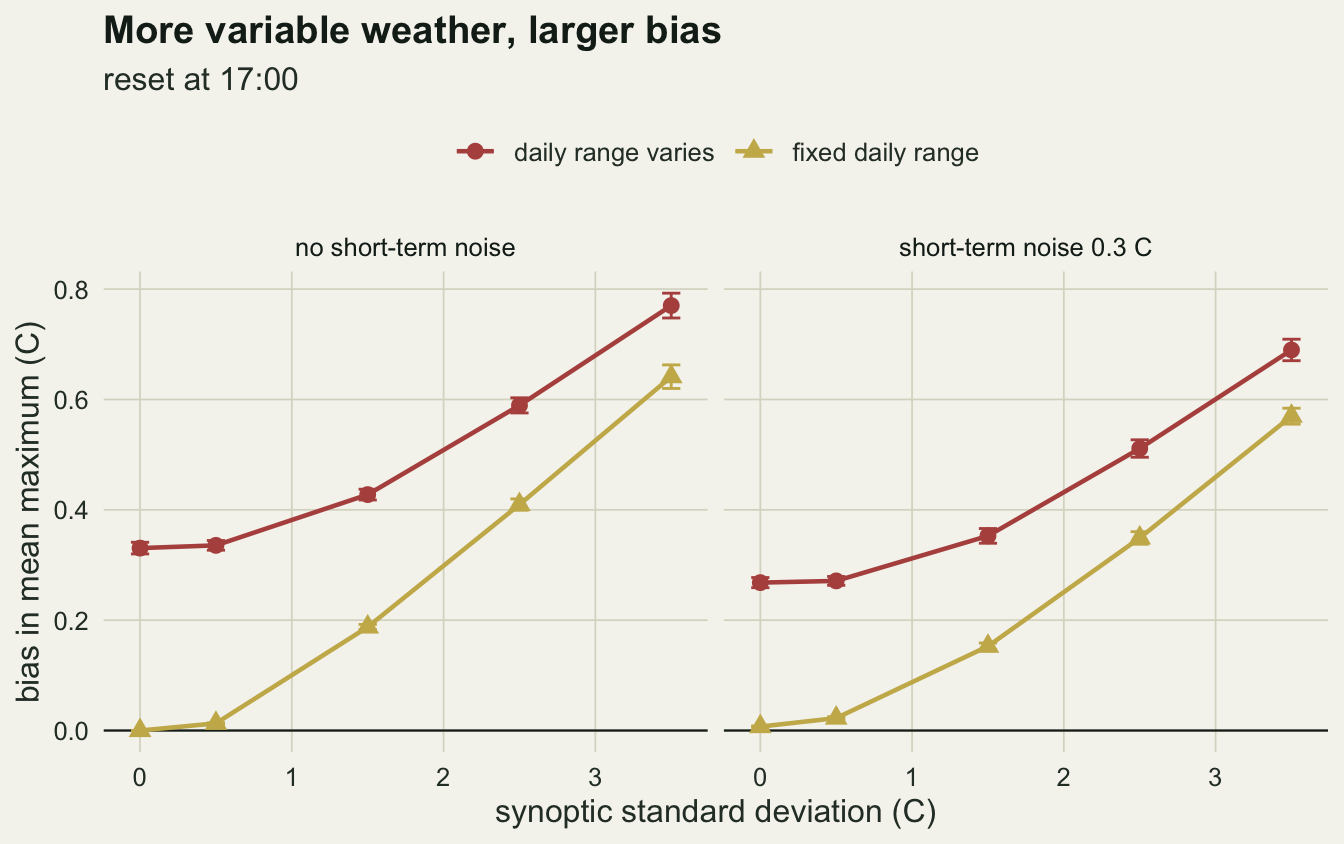
What a borrowed correction repairs
For a logger the repair is trivial: summarise the raw values by calendar day and the bias is gone, whatever hour the logger was downloaded. For a notebook of thermometer readings the raw values do not exist, and the usual route is a correction estimated from hourly data. Karl and colleagues (1986) fitted an empirical model to hourly records from 79 stations that predicts the monthly bias for a given observation hour, with the day-to-day temperature change and the solar geometry that shapes the daily range among its inputs, so that it could be applied at stations with no hourly record. Three simplified versions are compared here, each subtracting a monthly mean bias from the 17:00 maximum of the main station.
The local version uses 5 years of a 10-minute logger at the same site: it shares the weather series but has its own daily ranges and noise. The borrowed version uses 5 years of a logger in a climate with synoptic standard deviation 0.5 C, a maritime site. The scaled version fits a straight line of bias against the standard deviation of the day-to-day change in the maximum over the grid cells with varying range and noise, leaving out the 2.5 C cell, and predicts the main station’s bias from that statistic computed on the notebook maximum itself. That last one is the closest of the three to the spirit of a regression correction: it needs only the biased record and a relation fitted elsewhere. For the same reason the line is fitted on the statistic taken from the grid cells’ own 17:00 records, not from their calendar maxima, since a relation built at hourly stations and applied to observer records has to use a predictor both can supply; the section also shows what the calendar version would do.
set.seed(4421)
month_of <- function(day) pmin(12, floor(((day - 1) %% 365) / (365 / 12)) + 1)
monthly_bias <- function(stn, last_years = 5) {
  ext <- reset_extremes(stn, 17)
  keep <- ext$day > (n_years - last_years) * 365
  tapply(ext$obs_max[keep] - ext$cal_max[ext$day[keep]], month_of(ext$day[keep]), mean)
}
local_logger <- make_station(weather_main)
maritime_logger <- make_station(make_weather(0.5))
corr_local <- monthly_bias(local_logger)
corr_borrow <- monthly_bias(maritime_logger)

fit_rows <- grid_res[grid_res$amp == main_amp & grid_res$noise == main_noise & grid_res$syn != main_syn, ]
scale_fit <- lm(tmax ~ dtd_obs, data = fit_rows)
dtd_notebook <- sd(diff(ext17$obs_max))
corr_scaled <- predict(scale_fit, newdata = data.frame(dtd_obs = dtd_notebook))
dtd_calendar <- sd(diff(ext17$cal_max))
# the mismatched version: line fitted on calendar variability, fed the notebook statistic
scale_fit_cal <- lm(tmax ~ dtd_cal, data = fit_rows)
corr_mismatch <- predict(scale_fit_cal, newdata = data.frame(dtd_cal = dtd_notebook))
corr_cal_cal <- predict(scale_fit_cal, newdata = data.frame(dtd_cal = dtd_calendar))
mismatch_left <- mean(ext17$obs_max - corr_mismatch - ext17$cal_max[ext17$day])
dtd_ratio <- with(grid_res[grid_res$amp == main_amp & grid_res$syn > 0, ], range(dtd_obs / dtd_cal))

d17 <- ext17$day
hot_thr_main <- quantile(ext17$cal_max, hot_q, names = FALSE)
repaired <- list("no correction" = ext17$obs_max,
                 "local logger" = ext17$obs_max - corr_local[month_of(d17)],
                 "maritime logger" = ext17$obs_max - corr_borrow[month_of(d17)],
                 "scaled by variability" = ext17$obs_max - corr_scaled,
                 "07:00 reset instead" = ext07$obs_max)
repair_tab <- do.call(rbind, lapply(names(repaired), function(nm) {
  x <- repaired[[nm]]; err <- x - ext17$cal_max[d17]
  data.frame(method = nm, bias = mean(err),
             se = sd(tapply(err, (d17 - 1) %/% 365, mean)) / sqrt(n_years),
             hot_ratio = sum(x > hot_thr_main) / sum(ext17$cal_max[d17] > hot_thr_main),
             hot_hit = sum(x > hot_thr_main & ext17$cal_max[d17] > hot_thr_main) /
               sum(ext17$cal_max[d17] > hot_thr_main),
             day_rmse = sqrt(mean(err^2)))
}))
rmse_07_shift <- sqrt(mean((ext07$obs_max[-1] - ext07$cal_max[ext07$day[-1] - 1])^2))
share_07_equal <- mean(abs(ext07$obs_max[-1] - ext07$cal_max[ext07$day[-1] - 1]) < 1e-9)
rp <- function(nm, col) repair_tab[repair_tab$method == nm, col]
repair_tab$method <- factor(repair_tab$method, levels = rev(names(repaired)))
The uncorrected 17:00 maximum is +0.52 C too warm with 1.19 times the calendar count of hot days. The local correction brings the mean to -0.006 C and the hot-day ratio to 0.98. The maritime correction removes only part of the bias, leaving +0.24 C, because the maritime logger’s own bias was +0.28 C against the local +0.53 C. The scaled correction predicts +0.52 C and leaves -0.003 C, with a hot-day ratio of 0.99: within this model a relation fitted on four other climates transfers to the main station as well as a logger at the site does. It transfers only because the predictor is the same kind of statistic at both ends. The day-to-day standard deviation of the notebook maximum is 1.79 C against 2.26 C for the calendar maximum, because a carried-over afternoon replaces a cooler day with a copy of a warmer one and smooths the series; in every grid cell with varying range and some synoptic variation the notebook value is between 0.76 and 0.80 of the calendar value. A line fitted on calendar variability predicts +0.52 C when given the calendar statistic, which a notebook station cannot supply, but only +0.36 C when given the notebook statistic, and that version leaves +0.16 C of the bias in place.
A correct count does not mean the right days. After the local correction a share of 0.87 of the calendar hot days are also hot in the corrected record, and after the scaled correction 0.87: subtracting a constant pulls down days that were right along with days that were double-counted, so some true hot days drop below the threshold while some carried-over afternoons stay above it. The day-level error changes little under any of the three corrections: its root mean square falls from 1.08 C uncorrected to 0.95 C after the local correction and 0.95 C after the scaled one, since the error sits on particular days and a constant cannot find them. The 07:00 record has no mean bias in the maximum but a root mean square error of 2.26 C against the calendar day it is filed under, because a morning reading of the maximum describes the previous afternoon; filed under the previous day its root mean square error is 0.000 C, and it equals the previous calendar day’s maximum on a share of 1.000 of days.
Changing the observer from 17:00 to 07:00 part-way through a series is the case the splicing post treats. Here the step it would leave in the mean maximum is 0.52 C downward and in the mean minimum 0.49 C downward as well, with no change in climate, so the recorded diurnal range narrows by only 0.03 C while both columns shift; how much trend per decade that makes depends only on where the change falls, which is the arithmetic of that post.
p_bias <- ggplot(repair_tab, aes(bias, method)) +
  geom_vline(xintercept = 0, colour = te_ink, linewidth = 0.4) +
  geom_errorbar(aes(xmin = bias - 2 * se, xmax = bias + 2 * se), orientation = "y",
                width = 0.2, colour = te_body, linewidth = 0.5) +
  geom_point(size = 3, colour = te_rust) +
  labs(x = "bias in mean maximum (C)", y = NULL) +
  theme_datasheet()
hot_long <- rbind(data.frame(method = repair_tab$method, value = repair_tab$hot_ratio,
                             measure = "count, recorded / calendar"),
                  data.frame(method = repair_tab$method, value = repair_tab$hot_hit,
                             measure = "calendar hot days also hot"))
p_hot <- ggplot(hot_long, aes(value, method, colour = measure, shape = measure)) +
  geom_vline(xintercept = 1, colour = te_ink, linewidth = 0.4) +
  geom_point(size = 3) +
  scale_colour_manual(values = c("count, recorded / calendar" = te_forest,
                                 "calendar hot days also hot" = te_gold), name = NULL) +
  scale_shape_manual(values = c("count, recorded / calendar" = 16,
                                "calendar hot days also hot" = 17), name = NULL) +
  guides(colour = guide_legend(ncol = 1), shape = guide_legend(ncol = 1)) +
  labs(x = "hot days (ratio or share)", y = NULL) +
  theme_datasheet() +
  theme(axis.text.y = element_blank(), legend.position = "top")
(p_bias | p_hot) +
  plot_annotation(title = "A correction fixes the mean, not the individual days",
                  theme = theme_datasheet())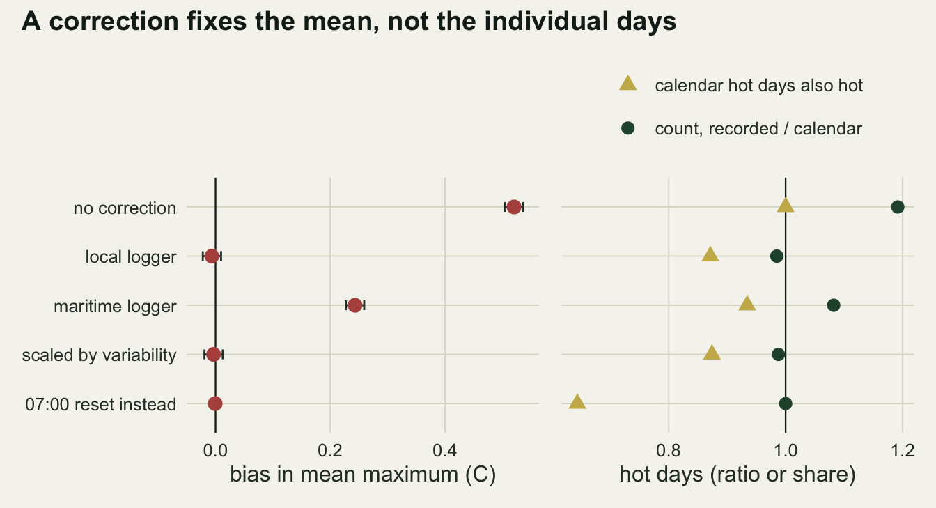
What to report
Report the observation or reset hour with any daily maximum and minimum, and for logger summaries say whether days run midnight to midnight. If the hour is unknown, say so; at the main station of this simulation not knowing whether the hour was 07:00 or 17:00 spans 0.52 C in the mean maximum and 0.49 C in the mean minimum, and any hour between them spans 0.80 C in the mean maximum.
If raw logger values exist, recompute daily extremes by calendar day rather than correcting the summaries. Apart from re-filing a morning-read maximum under the previous date, that is the only repair here that fixes individual days as well as the mean.
If a correction is applied to thermometer readings, report where the hourly data behind it came from and whether its predictor was computed on the same kind of record it is applied to. Treat analyses that depend on which days crossed a threshold (hot spells, the timing of a frost, degree days above a base accumulated to a date) as still affected after a mean correction: in this simulation the local correction took the hot-day ratio from 1.19 to 0.98, yet a share of only 0.87 of the calendar hot days were hot in the corrected record.
When two sites or two periods are compared, check whether their observation hours differ before reading a difference in heat accumulation as a difference in climate.
Honest limits
The diurnal cycle is a fixed shape with the minimum at 06:00 and the maximum at 15:00 all year, and the synoptic variance does not change with season. Real stations have later winter minima, shorter winter days, and larger day-to-day variability in winter at mid-latitudes, so the monthly corrections are flat here and seasonal in reality. The reset hours that look safe for both extremes in this model are a consequence of the shape and should not be taken as advice.
Weather is interpolated linearly between daily values. Fronts in reality arrive as faster changes, often with a preferred time of day, which alters the carry-over at particular hours; cloud and rain also cut an afternoon short in ways that a smooth range variation does not imitate.
The thermometer is perfect apart from the short-term noise. A real Six’s thermometer can have a sticking index, may not be reset properly, and is read by a person who rounds the reading; none of that is simulated, and the reset reading is taken to equal the air temperature at that instant.
The corrections are simplified. Karl and colleagues fitted their model to 79 hourly stations and checked it on 28 more; the scaled version here uses one predictor and four grid cells that differ from the main station only in synoptic variability, which is the easiest transfer a regression correction can face, and the maritime borrowed version is a single extreme case. Real climates also differ in the timing of the diurnal cycle, cloudiness and seasonality, and how far a regression correction transfers between them was not measured here.
Twenty years per cell is enough to see differences of a few hundredths of a degree in the mean, but the hot-day ratios carry their own Monte Carlo error that is not shown; at the main station a ratio rests on about 730 calendar hot days.
On whether afternoon readings matter today: the correction in the United States network exists because observation hours at cooperative stations shifted over the decades, and field stations that read a thermometer on a working-day visit do the same. Logger summaries over download-to-download days are a question of how a script was written, and they can be checked only when the script is available. The simulation does not measure how common either practice is.
References
Baker DG 1975 Journal of Applied Meteorology 14(4):471-476 (10.1175/1520-0450(1975)014<0471:EOOTOM>2.0.CO;2)
Karl TR, Williams CN, Young PJ, Wendland WM 1986 Journal of Climate and Applied Meteorology 25(2):145-160 (10.1175/1520-0450(1986)025<0145:AMTETT>2.0.CO;2)
Vose RS, Williams CN, Peterson TC, Karl TR, Easterling DR 2003 Geophysical Research Letters 30(20):2046 (10.1029/2003GL018111)
Menne MJ, Williams CN, Vose RS 2009 Bulletin of the American Meteorological Society 90(7):993-1008 (10.1175/2008BAMS2613.1)