library(ggplot2)

te_pal <- list(forest = "#275139", green = "#2f8f63", sage = "#93a87f",
               clay = "#b5534e", gold = "#cda23f", line = "#dad9ca",
               ink = "#16241d", paper = "#f5f4ee")

theme_te <- function() {
  theme_minimal(base_size = 12) +
    theme(panel.grid.minor = element_blank(),
          panel.grid.major = element_line(colour = "#e7e6dc"),
          plot.background = element_rect(fill = "#f5f4ee", colour = NA),
          panel.background = element_rect(fill = "#f5f4ee", colour = NA),
          plot.title = element_text(face = "bold", colour = te_pal$ink),
          axis.title = element_text(colour = "#2c3a31"))
}Degree days and thermal time in R
R
phenology
climate
thermal ecology
ecology tutorial
ggplot2
Build degree day models in R, compare the average, triangle and sine methods, estimate a base temperature from data, and measure what each choice costs.
A degree day model is the cheapest useful thing in phenology. It says that development is driven by warmth above a threshold, that the warmth adds up, and that the organism does whatever it does when a fixed total has accumulated. Two numbers a day, a minimum and a maximum, are enough to run it. Pest advisory services, irrigation schedules and crop calendars all rest on this arithmetic, and it works well enough that most people never look inside it.
Three choices sit inside it, and all three are routine enough to go unrecorded in the methods section. The base temperature below which nothing accumulates is usually taken from a paper about a different population. The arithmetic that turns a daily minimum and maximum into a day of heat comes in at least three versions that disagree. The date on which accumulation starts is a convention. This post measures what each choice is worth, in days of predicted event date, against a simulated organism whose true requirement is known exactly.
The setup assumes you have met a development rate curve before. If you have not, Thermal performance curves builds one and shows why the rate is a curve rather than a line. The reason a linear model of a curved response is not innocent once temperature varies within the day is Jensen’s inequality and thermal variability, and the last section of this post is that argument turned into a measurement.
The short version of what follows: the sophisticated daily method is the least accurate of the three here, all of the disagreement between two of the methods lives on a quarter of the days, the base temperature moves the predicted date more than four times as far as two degrees of warming does, and the standard way of estimating the base from data stops working when the organism’s own requirement varies by 5 per cent from year to year.
A day of temperature is not a triangle
To score a method you need a truth, and the truth here is a temperature curve rather than a pair of numbers. Each simulated day has a minimum at dawn and a maximum in mid afternoon. Between them the temperature rises along a quarter sine wave; after the maximum it decays exponentially towards the next morning’s minimum. That shape is the standard description of a clear day and it is deliberately asymmetric, because real days are: the temperature spends more of the twenty four hours near the bottom of its range than near the top.
The seasonal mean is a cosine with an annual amplitude of eleven degrees, the daily anomaly is a first order autoregressive process so that warm spells last several days, and the daily range is wider in summer than in spring. The organism starts accumulating on 1 March and develops when a known number of true degree days, integrated continuously above the true base, has gone by. Every number in this post is measured against that.
set.seed(20260719)

doy_start <- 32       # 1 February
n_day     <- 250      # season length in days
n_step    <- 96       # sub-daily steps
t_low     <- 5        # hour of the daily minimum
t_high    <- 15       # hour of the daily maximum
night_k   <- 2.4      # curvature of the overnight decay
phi_ano   <- 0.72     # day to day autocorrelation of the weather anomaly
sd_ano    <- 2.8      # standard deviation of the weather anomaly
tbase_true <- 8       # true base temperature
K_true    <- 700      # true requirement, degree days
biofix    <- 60       # 1 March: the day accumulation truly starts
n_pool    <- 300      # independent simulated years

season_doy <- doy_start + seq_len(n_day) - 1
win_idx    <- which(season_doy >= biofix)[1]

gen_year <- function() {
  nn <- n_day + 2
  dd <- doy_start - 2 + seq_len(nn)
  mu <- 11 + 11 * cos(2 * pi * (dd - 201) / 365)
  e <- numeric(nn)
  e[1] <- rnorm(1, 0, sd_ano)
  for (i in 2:nn) e[i] <- phi_ano * e[i - 1] + sqrt(1 - phi_ano^2) * rnorm(1, 0, sd_ano)
  hh <- pmax(1.5, 4.5 + 1.2 * cos(2 * pi * (dd - 201) / 365) + rnorm(nn, 0, 0.8))
  list(L = mu + e - hh, H = mu + e + hh)
}

night_frac <- function(s) (exp(-night_k * s) - exp(-night_k)) / (1 - exp(-night_k))

fine_temp <- function(yr, nstep = n_step) {
  idx <- 2:(n_day + 1)
  tt <- (seq_len(nstep) - 0.5) * 24 / nstep
  nl <- 24 - (t_high - t_low)
  out <- matrix(0, nrow = n_day, ncol = nstep)
  pre <- tt < t_low; rise <- tt >= t_low & tt <= t_high; post <- tt > t_high
  L <- yr$L; H <- yr$H
  flat <- function(k) rep(1, k)
  out[, pre] <- outer(L[idx], flat(sum(pre))) +
    outer(H[idx - 1] - L[idx], night_frac((tt[pre] + 24 - t_high) / nl))
  out[, rise] <- outer(L[idx], flat(sum(rise))) +
    outer(H[idx] - L[idx], sin(pi / 2 * (tt[rise] - t_low) / (t_high - t_low)))
  out[, post] <- outer(L[idx + 1], flat(sum(post))) +
    outer(H[idx] - L[idx + 1], night_frac((tt[post] - t_high) / nl))
  out
}

row_min <- function(m) m[cbind(seq_len(nrow(m)), max.col(-m, ties.method = "first"))]
row_max <- function(m) m[cbind(seq_len(nrow(m)), max.col(m, ties.method = "first"))]

pool_L <- matrix(0, n_pool, n_day + 2); pool_H <- pool_L
tmin_m <- matrix(0, n_pool, n_day); tmax_m <- tmin_m; true_dd <- tmin_m; tmean_m <- tmin_m
for (i in seq_len(n_pool)) {
  yy <- gen_year(); ff <- fine_temp(yy)
  pool_L[i, ] <- yy$L; pool_H[i, ] <- yy$H
  tmin_m[i, ] <- row_min(ff); tmax_m[i, ] <- row_max(ff)
  tmean_m[i, ] <- rowMeans(ff)
  true_dd[i, ] <- rowSums(pmax(ff - tbase_true, 0)) / n_step
}
true_dd[, seq_len(win_idx - 1)] <- 0

ff1 <- fine_temp(list(L = pool_L[1, ], H = pool_H[1, ]))
ff1_fine <- fine_temp(list(L = pool_L[1, ], H = pool_H[1, ]), nstep = 960)
tot_96  <- sum((rowSums(pmax(ff1 - tbase_true, 0)) / n_step)[win_idx:n_day])
tot_960 <- sum((rowSums(pmax(ff1_fine - tbase_true, 0)) / 960)[win_idx:n_day])

round(c(years = n_pool, season_days = n_day, steps_per_day = n_step,
        minutes_per_step = 24 * 60 / n_step, hour_of_minimum = t_low,
        hour_of_maximum = t_high, night_decay_k = night_k,
        weather_sd = sd_ano, weather_autocorrelation = phi_ano,
        true_base = tbase_true, true_requirement = K_true,
        first_doy = doy_start, biofix_doy = biofix), 2)
years season_days steps_per_day
300.00 250.00 96.00
minutes_per_step hour_of_minimum hour_of_maximum
15.00 5.00 15.00
night_decay_k weather_sd weather_autocorrelation
2.40 2.80 0.72
true_base true_requirement first_doy
8.00 700.00 32.00
biofix_doy
60.00 round(c(mean_tmin = mean(tmin_m[, win_idx:n_day]), mean_tmax = mean(tmax_m[, win_idx:n_day]),
mean_daily_range = mean((tmax_m - tmin_m)[, win_idx:n_day]),
midpoint_minus_true_mean = mean(((tmin_m + tmax_m) / 2 - tmean_m)[, win_idx:n_day])), 3) mean_tmin mean_tmax mean_daily_range
10.379 20.697 10.319
midpoint_minus_true_mean
0.341 round(c(integral_96_steps = tot_96, integral_960_steps = tot_960,
percent_gap = 100 * (tot_96 / tot_960 - 1)), 4) integral_96_steps integral_960_steps percent_gap
1953.4436 1953.4569 -0.0007 Across the 300 simulated seasons the mean daily minimum after 1 March is 10.379 degrees and the mean maximum is 20.697, a mean daily range of 10.319. One number in that block decides much of what follows: the midpoint of the daily extremes sits 0.341 degrees above the true daily mean. That gap is not a modelling artefact you can switch off. It follows from the shape of a day, and every method below starts by assuming the midpoint is the mean.
The continuous integral is computed at 96 steps a day. Recomputing one season at ten times that resolution moves the season total from 1953.4436 to 1953.4569 degree days, a gap of 0.0007 per cent, so the discretisation of the truth is not a source of any error reported here.
cross_from <- function(cs, dd, s, K) {
  offs <- if (s > 1) cs[s - 1] else 0
  tgt <- K + offs
  if (cs[length(cs)] < tgt) return(NA_real_)
  i <- which(cs >= tgt)[1]
  prev <- if (i == 1) 0 else cs[i - 1]
  (i - 1) + (tgt - prev) / dd[i]
}
cross_day <- function(dd, K, s = win_idx) cross_from(cumsum(dd), dd, s, K)
to_doy <- function(idx) idx + doy_start - 1

ev_true <- apply(true_dd, 1, cross_day, K = K_true)
round(c(mean_event_doy = mean(to_doy(ev_true)), sd_event_days = sd(ev_true),
        earliest_doy = min(to_doy(ev_true)), latest_doy = max(to_doy(ev_true))), 2)
mean_event_doy sd_event_days earliest_doy latest_doy
183.58 4.87 170.53 195.59 The event happens on day 183.58 of the year on average, with a standard deviation of 4.87 days and a range across the 300 years running from 170.53 to 195.59. That spread is pure weather: the requirement is fixed at 700 degree days and the organism has no variation of its own yet.
sel <- which(season_doy >= 88 & season_doy <= 108)
hour_mid <- (seq_len(n_step) - 0.5) * 24 / n_step
ser <- data.frame(
  day = rep(season_doy[sel], each = n_step) + rep(hour_mid / 24, length(sel)),
  temp = as.vector(t(ff1[sel, ])))
ser$top <- pmax(ser$temp, tbase_true)

ggplot(ser, aes(day, temp)) +
  geom_ribbon(aes(ymin = tbase_true, ymax = top), fill = te_pal$sage, alpha = 0.55) +
  geom_line(colour = te_pal$forest, linewidth = 0.35) +
  geom_hline(yintercept = tbase_true, colour = te_pal$clay, linewidth = 0.7) +
  scale_x_continuous(breaks = seq(90, 105, by = 5),
                     expand = expansion(mult = c(0.02, 0.02))) +
  labs(x = "Day of year", y = "Temperature (degrees C)",
       title = "The shaded area above the base line is the thermal time") +
  theme_te() +
  theme(plot.margin = margin(5.5, 12, 5.5, 5.5))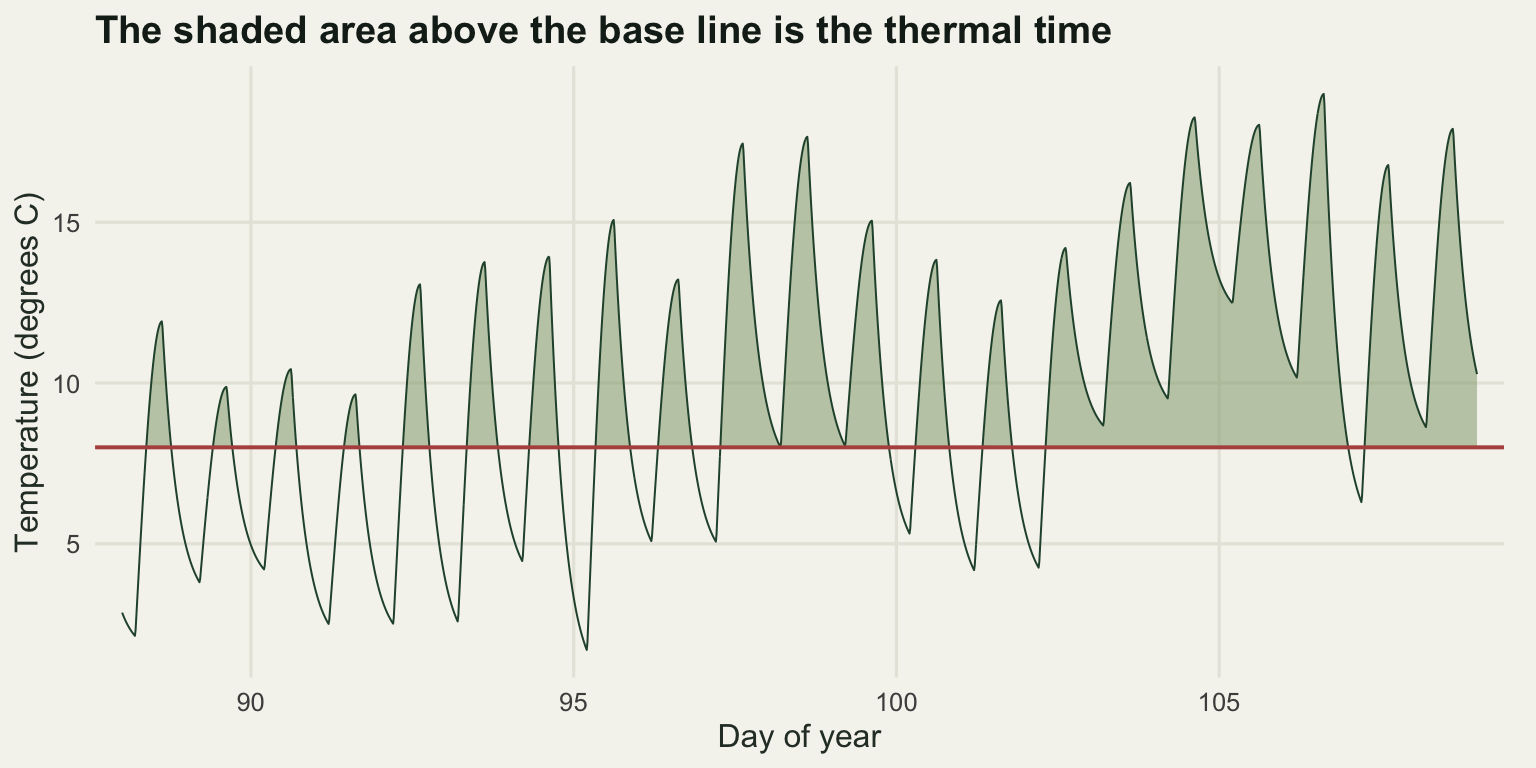
Three ways to turn two numbers into a day of heat
Nobody integrates a temperature curve. What arrives in a spreadsheet is a daily minimum and a daily maximum, and the three standard ways of turning that pair into a day of thermal time are all short enough to write by hand.
The simple average method takes the midpoint of the two extremes, subtracts the base and floors the result at zero:
\[DD = \max\left(0, \; \frac{T_{min} + T_{max}}{2} - T_b\right).\]
The single triangle method draws a straight line from the minimum up to the maximum and back again, and takes the area of that triangle above the base. When the base falls between the two extremes the area is a smaller triangle similar to the whole:
\[DD = \frac{(T_{max} - T_b)^2}{2\,(T_{max} - T_{min})}, \qquad T_{min} < T_b < T_{max}.\]
The single sine method of Baskerville and Emin replaces the triangle with half a sine wave through the same two extremes, and integrates the part of it above the base. Writing \(\bar{T} = (T_{max} + T_{min})/2\) for the midpoint and \(\alpha = (T_{max} - T_{min})/2\) for the half range, and setting \(\theta = \arcsin\!\left[(T_b - \bar{T})/\alpha\right]\), the day’s contribution when the base falls between the extremes is
\[DD = \frac{1}{\pi}\left[\left(\bar{T} - T_b\right)\left(\frac{\pi}{2} - \theta\right) + \alpha \cos\theta\right].\]
All three reduce to \(\bar{T} - T_b\) on a day whose minimum is already above the base, and all three give zero on a day whose maximum is below it. They can only differ on days that straddle the base, and the whole of the next section is about that.
dd_average <- function(tn, tx, tb) pmax((tn + tx) / 2 - tb, 0)

dd_triangle <- function(tn, tx, tb) {
  out <- pmax((tn + tx) / 2 - tb, 0)
  st <- tn < tb & tx > tb
  out[st] <- ((tx - tb)^2 / (2 * (tx - tn)))[st]
  out
}

dd_sine <- function(tn, tx, tb) {
  amp <- (tx - tn) / 2; avg <- (tx + tn) / 2
  out <- pmax(avg - tb, 0)
  st <- tn < tb & tx > tb
  th <- asin(pmin(1, pmax(-1, (tb - avg) / amp)))
  out[st] <- ((1 / pi) * ((avg - tb) * (pi / 2 - th) + amp * cos(th)))[st]
  out
}

mask <- function(m) { m[, seq_len(win_idx - 1)] <- 0; m }
dd_a <- mask(dd_average(tmin_m, tmax_m, tbase_true))
dd_t <- mask(dd_triangle(tmin_m, tmax_m, tbase_true))
dd_s <- mask(dd_sine(tmin_m, tmax_m, tbase_true))

tot <- function(m) rowSums(m)
season_tab <- rbind(
  total = c(truth = mean(tot(true_dd)), average = mean(tot(dd_a)),
            triangle = mean(tot(dd_t)), sine = mean(tot(dd_s))),
  pct_error = c(0, 100 * (mean(tot(dd_a)) / mean(tot(true_dd)) - 1),
                100 * (mean(tot(dd_t)) / mean(tot(true_dd)) - 1),
                100 * (mean(tot(dd_s)) / mean(tot(true_dd)) - 1)))
print(round(season_tab, 3))
truth average triangle sine
total 1751.842 1796.295 1815.983 1826.115
pct_error 0.000 2.538 3.661 4.240ev_a <- apply(dd_a, 1, cross_day, K = K_true)
ev_t <- apply(dd_t, 1, cross_day, K = K_true)
ev_s <- apply(dd_s, 1, cross_day, K = K_true)
date_tab <- rbind(
mean_doy = c(truth = mean(to_doy(ev_true)), average = mean(to_doy(ev_a)),
triangle = mean(to_doy(ev_t)), sine = mean(to_doy(ev_s))),
mean_days_from_truth = c(0, mean(ev_a - ev_true), mean(ev_t - ev_true),
mean(ev_s - ev_true)),
worst_year_days = c(0, max(abs(ev_a - ev_true)), max(abs(ev_t - ev_true)),
max(abs(ev_s - ev_true))))
print(round(date_tab, 3)) truth average triangle sine
mean_doy 183.58 183.024 181.666 180.981
mean_days_from_truth 0.00 -0.556 -1.914 -2.599
worst_year_days 0.00 2.072 4.174 5.087The season totals run the wrong way round. The continuous truth is 1751.842 degree days. The simple average returns 1796.295, which is 2.538 per cent high. The single triangle returns 1815.983, or 3.661 per cent high. The single sine, the method with the best physical justification, returns 1826.115 and is 4.24 per cent high, the worst of the three.
The predicted dates follow the same order. Against a true mean of day 183.58, the simple average predicts 183.024, the triangle 181.666 and the sine 180.981. In days that is 0.556, 1.914 and 2.599 early. In the single worst year of the 300 the errors are 2.072, 4.174 and 5.087 days.
That is not the ranking any textbook gives, and it is worth being precise about why it happens rather than filing it as noise. Two separate errors are in play. Every method assumes the daily mean is the midpoint of the extremes, and the midpoint sits 0.341 degrees too high, so every method over-accumulates on average. On top of that, the simple average throws away the warm hours of any day whose minimum is below the base, so it under-accumulates in early spring. The triangle and the sine recover those hours. They fix the second error and leave the first one untouched, which moves them further from the truth, not closer. The simple average wins here by cancellation, and cancellation is a property of this climate rather than of the method.
yr <- 1
panel_lv <- c("Accumulated thermal time", "Difference from the truth")
meth_lv <- c("Continuous truth", "Simple average", "Single triangle", "Single sine")
cum_mat <- cbind(cumsum(true_dd[yr, ]), cumsum(dd_a[yr, ]),
                 cumsum(dd_t[yr, ]), cumsum(dd_s[yr, ]))
keep <- season_doy >= biofix
acc_df <- do.call(rbind, lapply(seq_along(meth_lv), function(j)
  data.frame(doy = season_doy[keep], value = cum_mat[keep, j], method = meth_lv[j],
             panel = panel_lv[1])))
dif_df <- do.call(rbind, lapply(seq_along(meth_lv), function(j)
  data.frame(doy = season_doy[keep], value = (cum_mat[, j] - cum_mat[, 1])[keep],
             method = meth_lv[j], panel = panel_lv[2])))
acc_long <- rbind(acc_df, dif_df)
acc_long$panel <- factor(acc_long$panel, levels = panel_lv)
acc_long$method <- factor(acc_long$method, levels = meth_lv)
cross_pts <- data.frame(
  doy = to_doy(c(ev_true[yr], ev_a[yr], ev_t[yr], ev_s[yr])),
  value = K_true, method = factor(meth_lv, levels = meth_lv),
  panel = factor(panel_lv[1], levels = panel_lv))
req_line <- data.frame(yv = K_true, panel = factor(panel_lv[1], levels = panel_lv))

ggplot(acc_long, aes(doy, value, colour = method)) +
  geom_hline(data = req_line, aes(yintercept = yv), colour = te_pal$ink,
             linetype = "22", linewidth = 0.6) +
  geom_line(linewidth = 0.8) +
  geom_point(data = cross_pts, size = 2.4) +
  facet_wrap(~panel, ncol = 1, scales = "free_y") +
  scale_colour_manual(values = c(te_pal$ink, te_pal$green, te_pal$gold, te_pal$clay),
                      name = NULL) +
  labs(x = "Day of year", y = "Degree days",
       title = "The methods separate on the days that straddle the base") +
  theme_te() +
  theme(legend.position = "top",
        strip.text = element_text(colour = te_pal$ink, face = "bold"))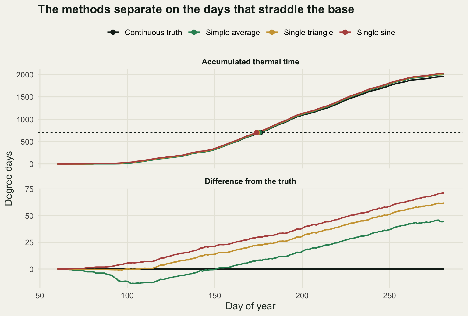
Where the disagreement lives, exactly
The claim in the last section was that the methods can only differ on days whose minimum is below the base and whose maximum is above it. That is a claim about arithmetic, so it can be checked rather than argued.
strad <- tmin_m < tbase_true & tmax_m > tbase_true
strad[, seq_len(win_idx - 1)] <- FALSE
gap <- dd_s - dd_a
round(c(straddle_days_per_year = mean(rowSums(strad)),
        window_days = n_day - win_idx + 1,
        straddle_share_of_days = 100 * mean(rowSums(strad)) / (n_day - win_idx + 1),
        total_gap_per_year = mean(rowSums(gap)),
        share_of_gap_on_straddle_days = 100 * sum(gap[strad]) / sum(gap),
        mean_gap_straddle_days = mean(gap[strad]),
        mean_gap_other_days = mean(gap[!strad]),
        largest_single_day_gap = max(gap)), 4)
straddle_days_per_year window_days
55.3000 222.0000
straddle_share_of_days total_gap_per_year
24.9099 29.8200
share_of_gap_on_straddle_days mean_gap_straddle_days
100.0000 0.5392
mean_gap_other_days largest_single_day_gap
0.0000 2.0798 tri_gap <- dd_t - dd_a
round(c(share_of_triangle_gap_on_straddle_days = 100 * sum(tri_gap[strad]) / sum(tri_gap),
mean_triangle_gap_straddle_days = mean(tri_gap[strad]),
mean_doy_of_straddle_days = sum(strad * matrix(season_doy, n_pool, n_day,
byrow = TRUE)) / sum(strad)), 4)share_of_triangle_gap_on_straddle_days mean_triangle_gap_straddle_days
100.000 0.356
mean_doy_of_straddle_days
120.659 mid_bias <- mask((tmin_m + tmax_m) / 2 - tmean_m)
round(c(mean_midpoint_bias_per_day = mean(mid_bias[, win_idx:n_day]),
bias_degree_days_to_event = mean(sapply(seq_len(n_pool), function(i) {
k <- floor(ev_true[i]); sum(mid_bias[i, seq_len(k)]) })),
as_percent_of_requirement = 100 * mean(sapply(seq_len(n_pool), function(i) {
k <- floor(ev_true[i]); sum(mid_bias[i, seq_len(k)]) })) / K_true), 3)mean_midpoint_bias_per_day bias_degree_days_to_event
0.341 35.880
as_percent_of_requirement
5.126 A season contains 222 days after the start date, and 55.3 of them straddle the base, which is 24.9099 per cent of the season. The mean difference between the sine method and the simple average over a whole season is 29.82 degree days. The share of that difference falling on straddle days is 100 per cent, and the mean difference on every other day is 0. Not approximately zero: exactly zero, on every non-straddle day of every one of the 300 years.
The reason is in the formulae. If the minimum is at or above the base, both methods return \(\bar{T} - T_b\); if the maximum is at or below the base, both return zero. There is no third case. The same holds for the triangle, whose difference from the simple average is also 100 per cent concentrated on straddle days. On the days where they do differ, the sine method adds 0.5392 degree days and the triangle adds 0.356, with a largest single day difference of 2.0798. The mean day of year of a straddle day is 120.659, which is the end of April: this is a spring phenomenon, and the further into the season you go the less any of it matters.
The other error does not behave that way. The midpoint of the extremes exceeds the true daily mean by 0.341 degrees on average, and unlike the straddle correction that gap lasts all season and never cancels. Summed from the start date to the event it comes to 35.88 degree days, which is 5.126 per cent of the requirement. That is the error the choice of daily method does nothing about, and it is larger than the error the choice of daily method fixes.
Choosing the base moves the date further than the climate does
The base temperature is the parameter nobody measures. A published thermal requirement for a species comes with a base attached, and the pair travels together into the next study, then into the study after that, where the climate is different and the population may be too. The sweep below asks what the assumed base is worth if the requirement is inherited as written, which is the ordinary case, and then what it is worth if you can recalibrate the requirement yourself.
bseq <- seq(4, 12, by = 0.5)
sweep_fixed <- sapply(bseq, function(b) {
  m <- mask(dd_sine(tmin_m, tmax_m, b))
  mean(to_doy(apply(m, 1, cross_day, K = K_true)))
})
cal_yr <- 1:20; test_yr <- 21:n_pool
sweep_recal <- t(sapply(bseq, function(b) {
  m <- mask(dd_sine(tmin_m, tmax_m, b))
  cs <- t(apply(m, 1, cumsum))
  acc <- sapply(seq_len(n_pool), function(i) {
    k <- floor(ev_true[i])
    cs[i, k] - cs[i, win_idx - 1] + (ev_true[i] - k) * m[i, k + 1]
  })
  req <- mean(acc[cal_yr])
  c(requirement = req,
    mean_doy = mean(to_doy(sapply(test_yr, function(i)
      cross_from(cs[i, ], m[i, ], win_idx, req)))))
}))
warm_shift <- 2
m8 <- mask(dd_sine(tmin_m, tmax_m, tbase_true))
m8w <- mask(dd_sine(tmin_m + warm_shift, tmax_m + warm_shift, tbase_true))
doy_base <- mean(to_doy(apply(m8, 1, cross_day, K = K_true)))
doy_warm <- mean(to_doy(apply(m8w, 1, cross_day, K = K_true)))

print(round(data.frame(base = bseq, published_requirement = sweep_fixed,
                       recalibrated = sweep_recal[, "mean_doy"],
                       requirement = sweep_recal[, "requirement"]), 2))
base published_requirement recalibrated requirement
1 4.0 157.14 183.47 1128.57
2 4.5 159.90 183.47 1075.03
3 5.0 162.70 183.47 1022.58
4 5.5 165.58 183.47 971.26
5 6.0 168.57 183.47 921.11
6 6.5 171.60 183.48 872.21
7 7.0 174.65 183.48 824.63
8 7.5 177.80 183.50 778.42
9 8.0 180.98 183.52 733.60
10 8.5 184.30 183.55 690.15
11 9.0 187.76 183.58 648.13
12 9.5 191.34 183.62 607.57
13 10.0 195.06 183.67 568.45
14 10.5 198.95 183.72 530.78
15 11.0 203.07 183.77 494.53
16 11.5 207.51 183.83 459.69
17 12.0 212.19 183.88 426.27swing_full <- diff(range(sweep_fixed))
swing_mid <- diff(range(sweep_fixed[bseq >= 6 & bseq <= 10]))
round(c(warming_degrees = warm_shift, calibration_years = length(cal_yr),
prediction_years = length(test_yr),
swing_base_4_to_12 = swing_full,
swing_base_6_to_10 = swing_mid,
swing_when_recalibrated = diff(range(sweep_recal[, "mean_doy"])),
baseline_doy = doy_base, warmed_doy = doy_warm,
warming_shift_days = doy_base - doy_warm,
ratio_full = swing_full / (doy_base - doy_warm),
ratio_mid = swing_mid / (doy_base - doy_warm)), 3) warming_degrees calibration_years prediction_years
2.000 20.000 280.000
swing_base_4_to_12 swing_base_6_to_10 swing_when_recalibrated
55.049 26.485 0.413
baseline_doy warmed_doy warming_shift_days
180.981 168.571 12.410
ratio_full ratio_mid
4.436 2.134 With the requirement held at its published value of 700 degree days, an assumed base of 4 puts the event on day 157.14 and an assumed base of 12 puts it on day 212.19. The swing is 55.049 days. Narrow the sweep to the range two papers on the same species might plausibly disagree over, 6 to 10 degrees, and the swing is still 26.485 days.
Set that against the climate signal the same model produces. Add 2 degrees uniformly to every temperature, keep the base at its true value of 8 and the requirement at 700, and the predicted date moves from 180.981 to 168.571, an advance of 12.41 days. The base sweep is 4.436 times that shift across the full range and 2.134 times it across the narrow one. A disagreement about a parameter that is almost never measured outweighs two degrees of warming in the answer, twice over even at the narrow end.
Now the honest half of the result, which came out differently from the way I expected. Recalibrate the requirement at each candidate base, using 20 calibration years and predicting the remaining 280, and the sweep almost vanishes: the predicted date runs from 183.47 at a base of 4 to 183.88 at a base of 12, a swing of 0.413 days. The recalibrated requirement is doing the work, moving from 1128.57 degree days at a base of 4 to 426.27 at a base of 12 to compensate.
The base temperature is therefore not dangerous on its own. It is dangerous because it arrives welded to a requirement calibrated at some other base, and the pair is only meaningful together. A paper that reports a requirement without its base has reported nothing; a study that adopts a base from the literature and a requirement from elsewhere has combined two numbers that were never about the same quantity. If you have several years of your own observations, recalibrating at whatever base you like costs almost nothing in accuracy, which is a more useful conclusion than the headline swing.
sseq <- seq(32, 92, by = 4)
start_tab <- sapply(c(4, 6, 8), function(b) {
  m <- dd_sine(tmin_m, tmax_m, b)
  cs <- t(apply(m, 1, cumsum))
  sapply(sseq, function(s) {
    si <- s - doy_start + 1
    mean(to_doy(sapply(seq_len(n_pool), function(i) cross_from(cs[i, ], m[i, ], si, K_true))))
  })
})
dimnames(start_tab) <- list(paste0("start_doy_", sseq), paste0("base_", c(4, 6, 8)))
print(round(start_tab, 2))
base_4 base_6 base_8
start_doy_32 156.17 168.20 180.88
start_doy_36 156.26 168.23 180.88
start_doy_40 156.36 168.26 180.89
start_doy_44 156.47 168.31 180.90
start_doy_48 156.58 168.35 180.92
start_doy_52 156.72 168.41 180.93
start_doy_56 156.92 168.48 180.95
start_doy_60 157.14 168.57 180.98
start_doy_64 157.39 168.68 181.02
start_doy_68 157.72 168.85 181.08
start_doy_72 158.11 169.05 181.17
start_doy_76 158.62 169.33 181.30
start_doy_80 159.22 169.68 181.47
start_doy_84 159.91 170.09 181.69
start_doy_88 160.73 170.62 181.99
start_doy_92 161.68 171.26 182.38round(c(start_swing_base_8 = diff(range(start_tab[, "base_8"])),
start_swing_base_6 = diff(range(start_tab[, "base_6"])),
start_swing_base_4 = diff(range(start_tab[, "base_4"]))), 3)start_swing_base_8 start_swing_base_6 start_swing_base_4
1.502 3.061 5.507 The third routine choice is the date accumulation starts, and it turned out to be much cheaper than the other two. Moving the start from 1 February to 2 April, a span of two months, moves the predicted date by 1.502 days at a base of 8. That is the whole effect. Winter days simply do not have maxima above 8 degrees often enough to matter, so almost nothing accumulates before the true start whatever you do.
The size of that effect is not a constant, though, and the table shows what it depends on. At a base of 6 the same sweep of start dates is worth 3.061 days, and at a base of 4 it is worth 5.507. The lower the base, the more of the winter counts, and the more the arbitrary start date decides the answer. In a warmer climate, or for a species with a base near freezing, the start date would be the expensive choice rather than the cheap one. It is cheap here for a reason that can be stated and checked, not because start dates never matter.
kind_lv <- c("Requirement taken from the literature",
             "Requirement recalibrated at each base")
base_df <- data.frame(
  base = rep(bseq, 2),
  doy = c(sweep_fixed, sweep_recal[, "mean_doy"]),
  kind = factor(rep(kind_lv, each = length(bseq)), levels = kind_lv))
arrow_df <- data.frame(x = tbase_true, xend = tbase_true, y = doy_base, yend = doy_warm)

ggplot(base_df, aes(base, doy, colour = kind)) +
  geom_line(linewidth = 0.9) +
  geom_point(size = 1.7) +
  geom_segment(data = arrow_df, aes(x = x, xend = xend, y = y, yend = yend),
               inherit.aes = FALSE, colour = te_pal$ink, linewidth = 0.9,
               arrow = arrow(length = unit(0.16, "cm"), ends = "both")) +
  annotate("text", x = tbase_true + 0.25, y = (doy_base + doy_warm) / 2,
           label = "2 degrees of warming", hjust = 0, size = 3.4, colour = te_pal$ink) +
  scale_colour_manual(values = c(te_pal$clay, te_pal$forest), name = NULL) +
  labs(x = "Assumed base temperature (degrees C)", y = "Mean predicted event, day of year",
       title = "The base is only meaningful with its requirement attached") +
  theme_te() +
  theme(legend.position = "top")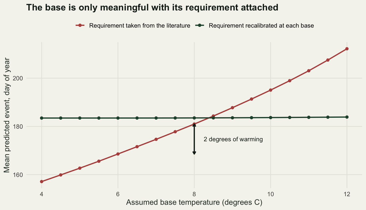
Estimating the base temperature from data
The standard repair is to estimate the base rather than assume it. The oldest and most widely used method takes several years of observed event dates, computes the accumulated thermal time to the event at each candidate base, and picks the base that makes those accumulations most consistent across years, measured by the coefficient of variation. If the base is right the organism needs the same total every year, so the coefficient of variation should be small; if it is wrong, warm years and cold years require different totals.
bgrid <- seq(2, 14, by = 0.1)
wmat <- t(sapply(seq_len(n_pool), function(i) {
  k <- floor(ev_true[i]); w <- numeric(n_day)
  w[win_idx:k] <- 1; w[k + 1] <- ev_true[i] - k; w
}))
A_clean <- sapply(bgrid, function(b) rowSums(dd_sine(tmin_m, tmax_m, b) * wmat))
pick_base <- function(AA, rows, gg) {
  sub <- AA[rows, , drop = FALSE]
  mu <- colMeans(sub)
  sdv <- sqrt(colSums((sub - rep(mu, each = length(rows)))^2) / (length(rows) - 1))
  gg[which.min(sdv / mu)]
}
n_rep <- 400
ygrid <- c(3, 4, 5, 6, 8, 10, 15, 20, 30, 40)
set.seed(4104)
clean_tab <- t(sapply(ygrid, function(Y) {
  est <- replicate(n_rep, pick_base(A_clean, sample.int(n_pool, Y), bgrid))
  c(years = Y, mean = mean(est), bias = mean(est) - tbase_true, sd = sd(est))
}))
print(round(clean_tab, 4))
years mean bias sd
[1,] 3 8.2060 0.2060 1.1424
[2,] 4 8.4418 0.4418 0.7454
[3,] 5 8.3860 0.3860 0.6000
[4,] 6 8.3292 0.3293 0.4732
[5,] 8 8.3772 0.3773 0.3396
[6,] 10 8.4068 0.4068 0.2728
[7,] 15 8.3753 0.3753 0.2019
[8,] 20 8.3875 0.3875 0.1693
[9,] 30 8.3840 0.3840 0.1433
[10,] 40 8.3958 0.3957 0.1133hit <- which(clean_tab[, "sd"] < 0.5)[1]
round(c(replicates_per_row = n_rep, base_grid_low = min(bgrid), base_grid_high = max(bgrid),
base_grid_step = 0.1,
years_needed_for_sd_under_half = as.numeric(clean_tab[hit, "years"]),
sd_there = as.numeric(clean_tab[hit, "sd"]),
bias_there = as.numeric(clean_tab[hit, "bias"])), 3) replicates_per_row base_grid_low
400.000 2.000
base_grid_high base_grid_step
14.000 0.100
years_needed_for_sd_under_half sd_there
6.000 0.473
bias_there
0.329 Each row of that table is 400 replicate datasets, each one a fresh sample of years from the pool, with the base searched on a grid from 2 to 14 degrees in steps of 0.1. With 5 years of data the recovered base averages 8.386 with a standard deviation of 0.6. With 15 years it is 8.3753 with a standard deviation of 0.2019, and with 40 years 8.3958 with 0.1133. The standard deviation first falls below half a degree at 6 years, where it is 0.473.
That looks like a solved problem, and the bias column says it is not. The estimate does not converge on 8. It converges on about 8.4, and the offset does not shrink with more data: it is 0.329 at 6 years and 0.3957 at 40. More years buy precision about the wrong number.
bfine <- seq(6, 10, by = 0.25)
A_exact <- matrix(0, n_pool, length(bfine))
for (i in seq_len(n_pool)) {
  ff <- fine_temp(list(L = pool_L[i, ], H = pool_H[i, ]))
  for (j in seq_along(bfine)) {
    A_exact[i, j] <- sum((rowSums(pmax(ff - bfine[j], 0)) / n_step) * wmat[i, ])
  }
}
A_sine_f <- sapply(bfine, function(b) rowSums(dd_sine(tmin_m, tmax_m, b) * wmat))
set.seed(613)
src_tab <- t(sapply(c(15, 40), function(Y) {
  e1 <- replicate(200, pick_base(A_exact, sample.int(n_pool, Y), bfine))
  e2 <- replicate(200, pick_base(A_sine_f, sample.int(n_pool, Y), bfine))
  c(years = Y, exact_mean = mean(e1), exact_sd = sd(e1),
    sine_mean = mean(e2), sine_sd = sd(e2))
}))
print(round(src_tab, 4))
years exact_mean exact_sd sine_mean sine_sd
[1,] 15 8 0 8.3750 0.2199
[2,] 40 8 0 8.3938 0.1360The offset is worth chasing, because it is not the criterion’s fault. Repeat the whole exercise with the accumulation computed from the continuous temperature curve instead of from the daily sine approximation, and the criterion returns a base of exactly 8 with a standard deviation of 0 at both 15 and 40 years, because at the true base the accumulation to the event is exactly the same every year and the coefficient of variation is exactly zero. Run the same replicates through the sine approximation and the answer is 8.375 and 8.3938. The bias in the estimated base is inherited whole from the daily method used to compute the thermal time. An estimate of a base temperature is an estimate conditional on an arithmetic convention, and quoting one without the other repeats the mistake the previous section was about.
req_cv <- 0.05
set.seed(9110)
K_year <- K_true * exp(rnorm(n_pool, 0, req_cv))
ev_noisy <- sapply(seq_len(n_pool), function(i) cross_day(true_dd[i, ], K_year[i]))
w_noisy <- t(sapply(seq_len(n_pool), function(i) {
  k <- floor(ev_noisy[i]); w <- numeric(n_day)
  w[win_idx:k] <- 1; w[k + 1] <- ev_noisy[i] - k; w
}))
A_noisy <- sapply(bgrid, function(b) rowSums(dd_sine(tmin_m, tmax_m, b) * w_noisy))
set.seed(5150)
noisy_tab <- t(sapply(c(5, 15, 40), function(Y) {
  est <- replicate(n_rep, pick_base(A_noisy, sample.int(n_pool, Y), bgrid))
  c(years = Y, mean = mean(est), bias = mean(est) - tbase_true, sd = sd(est),
    at_floor = mean(est <= min(bgrid) + 1e-9))
}))
print(round(noisy_tab, 4))
years mean bias sd at_floor
[1,] 5 5.5665 -2.4335 3.7396 0.395
[2,] 15 4.5935 -3.4065 2.8707 0.455
[3,] 40 3.6623 -4.3378 2.1032 0.555cv_curve <- function(AA) apply(AA, 2, sd) / colMeans(AA)
cc_clean <- cv_curve(A_clean); cc_noisy <- cv_curve(A_noisy)
round(c(requirement_cv_percent = 100 * req_cv,
cv_at_true_base_clean = cc_clean[bgrid == tbase_true],
cv_minimum_clean = min(cc_clean), base_at_minimum_clean = bgrid[which.min(cc_clean)],
cv_at_true_base_noisy = cc_noisy[bgrid == tbase_true],
cv_at_lowest_base_noisy = cc_noisy[1],
base_at_minimum_noisy = bgrid[which.min(cc_noisy)],
event_sd_days_noisy = sd(ev_noisy)), 4) requirement_cv_percent cv_at_true_base_clean cv_minimum_clean
5.0000 0.0050 0.0044
base_at_minimum_clean cv_at_true_base_noisy cv_at_lowest_base_noisy
8.4000 0.0485 0.0461
base_at_minimum_noisy event_sd_days_noisy
2.0000 5.6579 Everything above gives the organism a requirement that never varies. Real ones vary. Give the requirement a lognormal year to year spread of 5 per cent, which is modest against published figures for insect development, and rerun the same estimator.
It collapses. With 5 years the recovered base averages 5.5665, a bias of 2.4335 degrees low, with a standard deviation of 3.7396, and 0.395 of the replicates return the bottom of the searched range. More data makes it worse rather than better: at 40 years the mean is 3.6623, the bias is 4.3378 degrees low, and 0.555 of replicates sit on the floor of the grid.
The mechanism is visible in the criterion itself. With a repeatable organism the coefficient of variation has a sharp interior minimum, 0.0044 at a base of 8.4 against 0.005 at the true base of 8. With 5 per cent biological noise the coefficient of variation at the true base is 0.0485 and at the lowest base on the grid it is 0.0461, and the minimum is at 2, the edge. The noise puts a floor under the numerator that no base can remove, while lowering the base inflates the denominator without limit. Minimising a ratio then means maximising the denominator, and the criterion slides downhill to wherever you stopped searching. An answer that lands on the edge of the search grid is the method telling you it has no interior minimum, which is worth checking for every time this estimator is run.
What thermal time cannot do: development is not linear
Everything so far granted the degree day model its central assumption: that development rate is a straight line in temperature above the base. It is not. Rate rises with temperature, peaks, and falls sharply beyond the peak, and every organism has such a curve. The question is what the linear approximation costs, and the answer depends on where the season sits relative to the peak.
The organism below is a slower stage that finishes in late summer, and its true development rate follows a Briere curve: proportional to \(T(T - T_0)\sqrt{T_L - T}\) between a lower threshold of 8 and an upper limit of 32, zero outside. A linear degree day model is fitted to it in the ordinary way, by calibrating a single requirement on 20 baseline years and applying it thereafter. Then the same organism is run through a hot year in which every temperature is 5 degrees above baseline.
T_low_dev <- 8; T_lethal <- 32; hot_shift <- 5; target_doy <- 225
n_dev <- 60
bri_shape <- function(tt) ifelse(tt > T_low_dev & tt < T_lethal,
                                 tt * (tt - T_low_dev) * sqrt(pmax(T_lethal - tt, 0)), 0)
tgrid <- seq(0, 36, by = 0.01)
t_opt <- tgrid[which.max(bri_shape(tgrid))]

S0 <- matrix(0, n_dev, n_day); S5 <- S0; D0 <- S0; D5 <- S0
hot_frac0 <- matrix(0, n_dev, n_day); hot_frac5 <- hot_frac0
for (i in seq_len(n_dev)) {
  ff <- fine_temp(list(L = pool_L[i, ], H = pool_H[i, ]))
  S0[i, ] <- rowSums(bri_shape(ff)) / n_step
  S5[i, ] <- rowSums(bri_shape(ff + hot_shift)) / n_step
  D0[i, ] <- rowSums(pmax(ff - tbase_true, 0)) / n_step
  D5[i, ] <- rowSums(pmax(ff + hot_shift - tbase_true, 0)) / n_step
  hot_frac0[i, ] <- rowMeans(ff > t_opt)
  hot_frac5[i, ] <- rowMeans((ff + hot_shift) > t_opt)
}
S0 <- mask(S0); S5 <- mask(S5); D0 <- mask(D0); D5 <- mask(D5)
acc_to <- function(dd, day) { k <- floor(day); sum(dd[seq_len(k)]) + (day - k) * dd[k + 1] }
target_idx <- target_doy - doy_start + 1
a_dev <- 1 / mean(apply(S0, 1, acc_to, day = target_idx))
t0 <- apply(S0 * a_dev, 1, cross_day, K = 1)
t5 <- apply(S5 * a_dev, 1, cross_day, K = 1)
acc0 <- sapply(seq_len(n_dev), function(i) acc_to(D0[i, ], t0[i]))
acc5 <- sapply(seq_len(n_dev), function(i) acc_to(D5[i, ], t5[i]))
K_dev <- mean(acc0[cal_yr])
p0 <- apply(D0, 1, cross_day, K = K_dev)
p5 <- apply(D5, 1, cross_day, K = K_dev)
dev_test <- 21:n_dev
err0 <- p0[dev_test] - t0[dev_test]
err5 <- p5[dev_test] - t5[dev_test]
hrs0 <- mean(sapply(dev_test, function(i) mean(hot_frac0[i, win_idx:floor(t0[i])])))
hrs5 <- mean(sapply(dev_test, function(i) mean(hot_frac5[i, win_idx:floor(t5[i])])))

brk <- seq(-15, 45, by = 1)
bin_of <- function(x) tabulate(findInterval(x, brk), nbins = length(brk) - 1)
hist0 <- numeric(length(brk) - 1); hist5 <- hist0
for (i in dev_test) {
  ff <- fine_temp(list(L = pool_L[i, ], H = pool_H[i, ]))
  hist0 <- hist0 + bin_of(ff[win_idx:floor(t0[i]), ])
  hist5 <- hist5 + bin_of(ff[win_idx:floor(t5[i]), ] + hot_shift)
}

round(c(lower_threshold = T_low_dev, upper_threshold = T_lethal,
        optimum_temperature = t_opt, hot_year_offset = hot_shift,
        target_completion_doy = target_doy,
        years_simulated = n_dev, calibration_years = length(cal_yr),
        test_years = length(dev_test), fitted_requirement = K_dev), 3)
lower_threshold upper_threshold optimum_temperature
8.000 32.000 26.540
hot_year_offset target_completion_doy years_simulated
5.000 225.000 60.000
calibration_years test_years fitted_requirement
20.000 40.000 1250.919 round(c(true_completion_normal_doy = mean(to_doy(t0[dev_test])),
true_completion_hot_doy = mean(to_doy(t5[dev_test])),
predicted_normal_doy = mean(to_doy(p0[dev_test])),
predicted_hot_doy = mean(to_doy(p5[dev_test])),
mean_error_normal_days = mean(err0), mean_error_hot_days = mean(err5),
mean_abs_error_normal = mean(abs(err0)), mean_abs_error_hot = mean(abs(err5)),
worst_year_hot = min(err5)), 3)true_completion_normal_doy true_completion_hot_doy
224.320 192.512
predicted_normal_doy predicted_hot_doy
224.405 185.639
mean_error_normal_days mean_error_hot_days
0.085 -6.873
mean_abs_error_normal mean_abs_error_hot
1.010 6.873
worst_year_hot
-13.196 round(c(hours_above_optimum_normal = 100 * hrs0, hours_above_optimum_hot = 100 * hrs5,
degree_days_used_normal = mean(acc0[dev_test]),
degree_days_used_hot = mean(acc5[dev_test]),
percent_more_in_hot_years = 100 * (mean(acc5[dev_test]) / mean(acc0[dev_test]) - 1),
cv_of_requirement_normal = sd(acc0[dev_test]) / mean(acc0[dev_test]),
cv_of_requirement_hot = sd(acc5[dev_test]) / mean(acc5[dev_test])), 3)hours_above_optimum_normal hours_above_optimum_hot
5.125 13.860
degree_days_used_normal degree_days_used_hot
1250.406 1378.608
percent_more_in_hot_years cv_of_requirement_normal
10.253 0.013
cv_of_requirement_hot
0.048 The optimum of that rate curve is at 26.54 degrees. In a normal year, 5.125 per cent of the hours between the start date and completion are above it. The linear model, calibrated on 20 years and tested on the remaining 40, is close to exact: the mean predicted date is 224.405 against a true 224.32, an error of 0.085 days, with a mean absolute error of 1.01 days. On a normal year the approximation is not merely adequate, it is very good.
In the hot year, 13.86 per cent of the development hours are above the optimum, and the model predicts day 185.639 against a true 192.512. That is 6.873 days early on average, with a worst year of 13.196 days early. The sign is the part that matters. The linear model believes that hotter is always faster, so it spends the extra warmth of a hot year on development that the organism does not actually achieve, and the prediction runs early. The error is not symmetric noise; it is a one-directional failure that arrives exactly when the summer is unusual.
The thermal constant itself gives the game away if you look. The organism uses 1250.406 degree days to complete in normal years and 1378.608 in hot ones, which is 10.253 per cent more, and the coefficient of variation of that supposedly constant requirement rises from 0.013 to 0.048. A requirement that changes with the weather is not a requirement. If your own calibration data show the accumulated total drifting upward in hot seasons, that is the linearity assumption breaking, not measurement error, and no amount of refitting the base or the requirement will repair it. The repair is a nonlinear rate model fitted to the whole curve.
This is the limit worth stating plainly. A degree day model is at its best in the years everyone finds unremarkable and at its worst in the years that get written up: heatwave years, range edge populations, and the warm end of a climate projection. Those are precisely the cases the model tends to be pointed at.
panel_r <- c("Development rate per day", "Share of development hours")
tp <- seq(0, 34, by = 0.05)
rate_df <- data.frame(
  temp = rep(tp, 2),
  value = c(a_dev * bri_shape(tp), pmax(tp - tbase_true, 0) / K_dev),
  series = factor(rep(c("True rate curve", "Linear degree day assumption"), each = length(tp)),
                  levels = c("True rate curve", "Linear degree day assumption")),
  panel = factor(panel_r[1], levels = panel_r))
mids <- brk[-length(brk)] + 0.5
keep_b <- mids >= -4 & mids <= 40
hist_df <- data.frame(
  temp = rep(mids[keep_b], 2),
  value = c((hist0 / sum(hist0))[keep_b], (hist5 / sum(hist5))[keep_b]),
  years = factor(rep(c("Normal years", "Hot years"), each = sum(keep_b)),
                 levels = c("Normal years", "Hot years")),
  panel = factor(panel_r[2], levels = panel_r))
opt_line <- data.frame(xv = t_opt, panel = factor(panel_r, levels = panel_r))

ggplot(mapping = aes(temp, value)) +
  geom_vline(data = opt_line, aes(xintercept = xv), colour = te_pal$ink,
             linetype = "22", linewidth = 0.6) +
  geom_col(data = hist_df, aes(fill = years), position = "identity",
           alpha = 0.6, width = 1) +
  geom_line(data = rate_df, aes(colour = series), linewidth = 0.9) +
  facet_wrap(~panel, ncol = 1, scales = "free_y") +
  scale_colour_manual(values = c(te_pal$forest, te_pal$clay), name = NULL) +
  scale_fill_manual(values = c(te_pal$sage, te_pal$gold), name = NULL) +
  coord_cartesian(xlim = c(0, 34)) +
  labs(x = "Temperature (degrees C)", y = NULL,
       title = "The linear model keeps rising where the organism slows down") +
  theme_te() +
  theme(legend.position = "top",
        strip.text = element_text(colour = te_pal$ink, face = "bold"))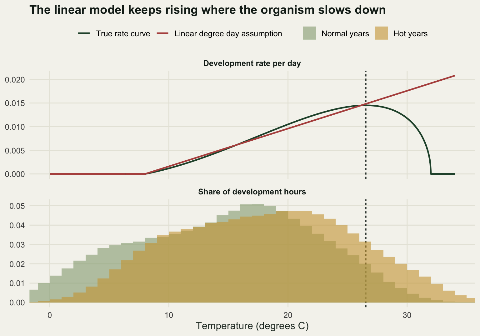
Where to go next
Thermal time is a good default and a bad final answer. It is worth keeping for the same reason a production model is worth keeping in a data poor fishery: it needs almost nothing and it is right often enough to be useful. What it needs is the discipline of reporting the base, the daily method and the start date together, because the results above show they are not independent conventions but three parts of one calibration. If the model is going to be used for warm years specifically, fit the rate curve instead, and see Thermal performance curves for how to do that and what it costs in data.
References
Baskerville GL, Emin P 1969 Ecology 50(3):514-517 (10.2307/1933912)
Trudgill DL, Honek A, Li D, Van Straalen NM 2005 Annals of Applied Biology 146(1):1-14 (10.1111/j.1744-7348.2005.04088.x)
Bonhomme R 2000 European Journal of Agronomy 13(1):1-10 (10.1016/S1161-0301(00)00058-7)
Yang S, Logan J, Coffey DL 1995 Agricultural and Forest Meteorology 74(1-2):61-74 (10.1016/0168-1923(94)02185-M)
Parton WJ, Logan JA 1981 Agricultural Meteorology 23:205-216 (10.1016/0002-1571(81)90105-9)