library(ggplot2)
options(scipen = 6)

te_pal <- list(forest = "#275139", green = "#2f8f63", sage = "#93a87f",
               clay = "#b5534e", gold = "#cda23f", line = "#dad9ca",
               ink = "#16241d", paper = "#f5f4ee")

theme_te <- function() {
  theme_minimal(base_size = 12) +
    theme(panel.grid.minor = element_blank(),
          panel.grid.major = element_line(colour = "#e7e6dc"),
          plot.background = element_rect(fill = "#f5f4ee", colour = NA),
          panel.background = element_rect(fill = "#f5f4ee", colour = NA),
          plot.title = element_text(face = "bold", colour = te_pal$ink),
          axis.title = element_text(colour = "#2c3a31"))
}Climate window analysis in R
R
climate
phenology
hypothesis testing
ecology tutorial
ggplot2
Slide every candidate weather window past a yearly ecological response in R, measure how often the naive best window is significant, and correct it properly.
You have a yearly number from a population: mean laying date, seed crop, the proportion of females that bred, emergence date. You also have a daily weather record, because someone runs a station nearby and the series goes back further than your fieldwork does. The biology responds to weather over some stretch of days, and you do not know which stretch. So you slide a window over the daily record, take the mean temperature inside it, regress the yearly response on that mean, and repeat for every start day and every window length you can think of. The window that fits best is the window you report.
That procedure is standard. It has a good R package behind it, it appears in a large number of published phenology and life history papers, and the reasoning is sound: you cannot fit a separate coefficient to all 365 days from 30 years of data, so you reduce the daily record to one number per year and let the data choose how. The trouble is the last step. The best window is chosen by a search over thousands of candidates, and then the p-value printed next to it is the p-value for a single regression that was specified in advance. Those are not the same quantity, and the gap between them is not a rounding error.
This post measures the gap. We simulate a daily weather series and a yearly response, so the true window is known and, in the null case, absent. Then we run the whole search on pure noise and count how often it comes back significant. We build the correct null by randomising the response across years and rerunning the entire search on each randomisation. We estimate how many independent tests the search really performs, which is far fewer than the nominal count, and we measure how precisely a window can be located when the effect is real.
If you have not fitted a response to temperature before, phenological trends and temperature covers the simpler version of the problem, where the window is fixed in advance by biology rather than chosen by fit. Everything below is the price of not fixing it.
A daily weather record and a yearly response
The weather is a seasonal cycle plus an autoregressive daily anomaly. Real daily temperature anomalies are strongly correlated from one day to the next, which matters here more than anything else about them: it is why neighbouring windows carry nearly the same information, and it is why the nominal number of tests is misleading. Day 1 of each record is 1 September of the preceding year, so the search covers the full 365 days before the biological measurement.
set.seed(20260719)

n_days <- 365
phi_day <- 0.8
sd_day <- 3
n_year <- 30

sim_weather <- function(nyr, ndays = n_days, phi = phi_day, sdd = sd_day) {
  x <- matrix(0, nyr, ndays)
  x[, 1] <- rnorm(nyr, 0, sdd)
  inn <- sdd * sqrt(1 - phi^2)
  for (d in 2:ndays) x[, d] <- phi * x[, d - 1] + rnorm(nyr, 0, inn)
  seasonal <- 9 + 9 * sin(2 * pi * (seq_len(ndays) - 230) / 365)
  x + matrix(seasonal, nyr, ndays, byrow = TRUE)
}

wx <- sim_weather(n_year)
anom <- wx - matrix(colMeans(wx), n_year, n_days, byrow = TRUE)
lag1 <- mean(sapply(seq_len(n_year), function(i)
  cor(anom[i, -n_days], anom[i, -1])))

print(round(c(years = n_year, days_per_year = n_days, target_phi = phi_day,
              measured_lag1 = lag1, anomaly_sd = sd(anom),
              coldest_day_mean = min(colMeans(wx)),
              warmest_day_mean = max(colMeans(wx))), 4))
years days_per_year target_phi measured_lag1
30.0000 365.0000 0.8000 0.7867
anomaly_sd coldest_day_mean warmest_day_mean
2.9271 -0.8076 19.3047 Thirty years of daily temperature, a seasonal mean running from -0.8076 to 19.3047 degrees, and anomalies with a standard deviation of 2.9271 degrees and a measured lag one autocorrelation of 0.7867 against the 0.8 we asked for. Thirty years is a good phenology dataset. Many published window analyses run on fewer.
The candidate windows are every start day on a two day grid crossed with every length from 10 to 180 days on a five day grid, keeping only those that end inside the record.
win_start <- seq(1, 356, by = 2)
win_len <- seq(10, 180, by = 5)
grid <- expand.grid(start = win_start, len = win_len)
grid <- grid[grid$start + grid$len - 1L <= n_days, ]
grid$end <- grid$start + grid$len - 1L
n_win <- nrow(grid)

print(c(candidate_starts = length(win_start), candidate_lengths = length(win_len),
        candidate_windows = n_win,
        shortest_window = min(grid$len), longest_window = max(grid$len)))
candidate_starts candidate_lengths candidate_windows shortest_window
178 35 4751 10
longest_window
180 win_means <- function(w) {
cs <- cbind(0, t(apply(w, 1, cumsum)))
(cs[, grid$start + grid$len, drop = FALSE] - cs[, grid$start, drop = FALSE]) /
rep(grid$len, each = nrow(w))
}
W <- win_means(wx)
print(round(c(rows = nrow(W), cols = ncol(W),
check_window_1 = W[1, 1],
check_by_hand = mean(wx[1, grid$start[1]:grid$end[1]])), 6)) rows cols check_window_1 check_by_hand
30.00000 4751.00000 13.74286 13.74286 That is 4751 candidate windows, from 178 start days and 35 lengths. A published search on every single start day and every single length would run to tens of thousands; ours is a coarser grid of the same object, and the conclusions below get milder, not sharper, for the coarseness.
The window means come from cumulative sums rather than from repeated averaging. Once you have the running total of the daily series, the mean of any window is one subtraction and one division, so the cost of the whole grid is the cost of one pass over the record. The check confirms it: window number one has a mean of 13.74286 by the cumulative sum route and 13.74286 computed directly. This is what makes the randomisation test below affordable, and it is why there is no excuse for skipping it.
What the search actually does
For each window we fit a straight line through the yearly response and keep the improvement in AIC over the intercept only model. For a single predictor and normal errors the improvement has a closed form, because the residual sum of squares of the fitted model is the residual sum of squares of the null model times one minus the R-squared:
\[\Delta \text{AIC} = -n \log \left( 1 - R^2 \right) - 2\]
with \(n\) the number of years. The ranking of windows by AIC improvement is therefore the ranking by R-squared, and both can be read off one call to cor. The identity is worth checking rather than believing.
r2_all <- function(y, Wm) as.vector(cor(y, Wm))^2
daic <- function(r2, n) -n * log1p(-r2) - 2
pnaive <- function(r2, n) pf(r2 * (n - 2) / (1 - r2), 1, n - 2, lower.tail = FALSE)

set.seed(11)
y_check <- rnorm(n_year)
j <- 500
m1 <- lm(y_check ~ W[, j])
m0 <- lm(y_check ~ 1)
print(round(c(formula_daic = daic(summary(m1)$r.squared, n_year),
              lm_daic = AIC(m0) - AIC(m1),
              formula_p = pnaive(summary(m1)$r.squared, n_year),
              lm_p = anova(m1)$`Pr(>F)`[1]), 8))
formula_daic lm_daic formula_p lm_p
2.778543 2.778543 0.036318 0.036318 The formula returns an AIC improvement of 2.778543 and lm returns 2.778543; the p-values agree at 0.036318. From here on the search runs through the formula, which costs one matrix multiplication for the whole grid.
Now put a real signal in. The response depends on the mean temperature over days 241 to 285, a 45 day window in late spring, and on nothing else. The coefficient is set so that the true window explains 35 per cent of the variance in the response, which is a strong but not absurd effect for a phenological trait.
true_start <- 241
true_len <- 45
true_end <- true_start + true_len - 1L
rho2 <- 0.35

set.seed(505)
pilot <- sim_weather(3000)
sd_w <- sd(rowMeans(pilot[, true_start:true_end]))
beta <- sqrt(rho2 / (1 - rho2)) / sd_w

make_y <- function(w, b = beta) {
  b * rowMeans(w[, true_start:true_end, drop = FALSE]) + rnorm(nrow(w))
}

print(round(c(true_start = true_start, true_end = true_end, true_len = true_len,
              target_R2 = rho2, target_R2_percent = 100 * rho2,
              sd_window_mean = sd_w, beta = beta), 4))
true_start true_end true_len target_R2
241.0000 285.0000 45.0000 0.3500
target_R2_percent sd_window_mean beta
35.0000 1.2764 0.5749 set.seed(707)
y_sig <- make_y(wx)
r2_sig <- r2_all(y_sig, W)
b_sig <- which.max(r2_sig)
near_best <- daic(r2_sig, n_year) >= daic(max(r2_sig), n_year) - 2
print(round(c(best_start = grid$start[b_sig], best_end = grid$end[b_sig],
best_len = grid$len[b_sig], best_R2 = max(r2_sig),
best_dAIC = daic(max(r2_sig), n_year),
best_p = pnaive(max(r2_sig), n_year),
R2_at_true_window = r2_sig[grid$start == true_start &
grid$len == true_len],
windows_within_2_AIC = sum(near_best),
near_start_span = diff(range(grid$start[near_best])),
near_length_span = diff(range(grid$len[near_best]))), 5)) best_start best_end best_len
249.00000 283.00000 35.00000
best_R2 best_dAIC best_p
0.38383 12.52718 0.00026
R2_at_true_window windows_within_2_AIC near_start_span
0.34764 22.00000 20.00000
near_length_span
40.00000 The search finds days 249 to 283 with an R-squared of 0.38383 and an AIC improvement of 12.52718. The truth is days 241 to 285. The recovered window is eight days late at its start, two days early at its end and ten days shorter, and it scores better than the true window does: 0.38383 against 0.34764. That last comparison is the whole problem in one line. The search is not looking for the true window, it is looking for the window that best fits this particular sample, and those differ by however much the noise happens to favour one over another.
surf <- data.frame(start = grid$start, len = grid$len,
                   dev = daic(r2_sig, n_year))
marks <- data.frame(start = c(true_start, grid$start[b_sig]),
                    len = c(true_len, grid$len[b_sig]),
                    kind = c("true window", "selected window"))

ggplot(surf, aes(start, len, fill = dev)) +
  geom_tile(width = 2, height = 5) +
  geom_point(data = marks, aes(start, len), inherit.aes = FALSE,
             shape = 21, fill = te_pal$paper, colour = te_pal$paper, size = 6) +
  geom_point(data = marks, aes(start, len, shape = kind), inherit.aes = FALSE,
             colour = te_pal$clay, size = 4.4, stroke = 1.8) +
  scale_fill_gradientn(colours = c("#cfcdb6", "#bcc5a1", "#a2b986",
                                   "#72a871", "#3a9366", "#275139"),
                       values = c(0, 0.08, 0.18, 0.35, 0.65, 1),
                       name = "AIC improvement") +
  scale_shape_manual(values = c("true window" = 1, "selected window" = 4),
                     name = NULL) +
  labs(x = "First day of the window", y = "Window length in days",
       title = "One dataset, 4751 candidate windows") +
  theme_te() +
  theme(legend.position = "right")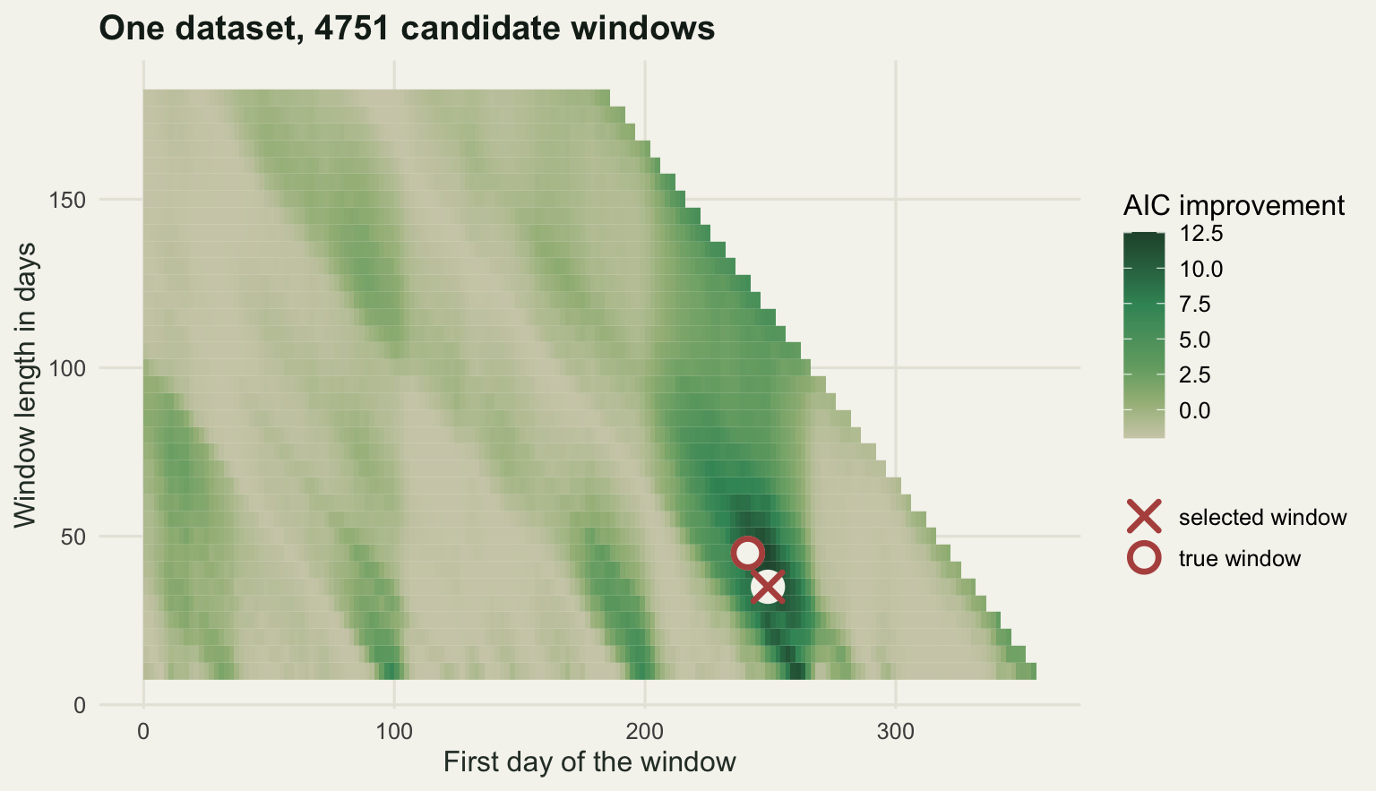
The surface is not a sharp peak on a flat plain. It is a diagonal ridge, because a window that shares most of its days with the best one shares most of its information, and because the weather inside it is autocorrelated anyway. The ridge runs along the set of windows that keep covering late spring while trading start day against length. Out of 4751 candidates, 22 sit within two AIC units of the winner, and those 22 spread over 20 days of start date and 40 days of length. Reporting the winner alone, with an interval computed as though it were the only window ever fitted, throws away the width of that ridge.
The same search on a response that is pure noise
Now delete the biology. The response is standard normal noise, generated without ever looking at the weather. There is no window. Run the identical search.
set.seed(9001)
wx0 <- sim_weather(n_year)
W0 <- win_means(wx0)
y0 <- rnorm(n_year)
r2_0 <- r2_all(y0, W0)
b0 <- which.max(r2_0)
print(round(c(null_best_start = grid$start[b0], null_best_end = grid$end[b0],
              null_best_R2 = max(r2_0), null_best_dAIC = daic(max(r2_0), n_year),
              null_best_p = pnaive(max(r2_0), n_year),
              null_median_R2 = median(r2_0),
              null_tests_under_05 = sum(pnaive(r2_0, n_year) < 0.05)), 5))
null_best_start null_best_end null_best_R2 null_best_dAIC
299.00000 313.00000 0.25472 6.82001
null_best_p null_median_R2 null_tests_under_05
0.00445 0.00931 39.00000 The search returns days 299 to 313, a two week window spanning the turn of June and July, with an R-squared of 0.25472, an AIC improvement of 6.82001 and a p-value of 0.00445. Written up, that reads as a clean result: a fortnight of midsummer temperature explains a quarter of the between year variance in the trait, p below one per cent. Every number in that sentence is correct, and the effect does not exist.
One realisation proves nothing. Repeat it 400 times, with a fresh weather record and a fresh noise response each time.
n_null <- 400
set.seed(1234)
null_run <- t(replicate(n_null, {
  ww <- sim_weather(n_year)
  rr <- r2_all(rnorm(n_year), win_means(ww))
  c(best = max(rr), hits = sum(pnaive(rr, n_year) < 0.05))
}))
null_best <- null_run[, "best"]
naive_fpr <- mean(pnaive(null_best, n_year) < 0.05)
print(round(c(replicates = n_null, naive_FPR = naive_fpr,
              naive_FPR_percent = 100 * naive_fpr,
              datasets_significant = sum(pnaive(null_best, n_year) < 0.05),
              median_best_R2 = median(null_best),
              q95_best_R2 = as.numeric(quantile(null_best, 0.95)),
              median_best_p = median(pnaive(null_best, n_year))), 5))
replicates naive_FPR naive_FPR_percent
400.00000 0.97500 97.50000
datasets_significant median_best_R2 q95_best_R2
390.00000 0.24201 0.38572
median_best_p
0.00576 print(round(c(expected_hits = 0.05 * n_win, mean_hits = mean(null_run[, "hits"]),
sd_hits = sd(null_run[, "hits"]),
min_hits = min(null_run[, "hits"]), max_hits = max(null_run[, "hits"]),
reps_with_no_hits = mean(null_run[, "hits"] == 0)), 2)) expected_hits mean_hits sd_hits min_hits
237.55 242.04 324.74 0.00
max_hits reps_with_no_hits
2083.00 0.03 The naive false positive rate is 0.975. In 390 of 400 datasets with no relationship whatsoever between weather and biology, the best window came back significant at the five per cent level. The median best R-squared under the null is 0.24201, the median best p-value is 0.00576, and one dataset in twenty produces a best window with an R-squared above 0.38572, which is larger than the effect we planted in the previous section.
This is the headline number of the post. A test that fires on 97.5 per cent of null datasets is not a weak test, it is not a test at all. It is a description of the searched grid.
The second block of numbers shows why counting tests will not repair it in the obvious way. Across the grid, 4751 windows at a five per cent level should produce 237.55 individually significant windows per dataset by chance, and the average over 400 datasets is 242.04, as it must be. The standard deviation of that count is 324.74. One dataset gave 2083 significant windows and three per cent of datasets gave none at all. The tests are not scattered independently across the grid: they arrive in clumps, because a run of warm years in the response either matches a broad region of the weather grid or matches nothing.
The correct null: randomise the response and rerun the whole search
The fix is old and simple. The thing that needs a null distribution is not one regression, it is the entire search procedure. So run the entire search on data where the null is true by construction. Break the link between the response and the weather by permuting the response across years, keeping the daily record exactly as it is, and record the best AIC improvement the search achieves. Repeat 500 times. The 95th percentile of those best values is the threshold the real best value has to beat.
Permuting the response and not the weather is the right choice here. It preserves every feature of the weather series, the seasonal cycle, the autocorrelation, the correlations between overlapping windows, and destroys only the association under test.
perm_best_r2 <- function(y, Wm, nperm) {
  n <- length(y)
  yc <- y - mean(y)
  Wc <- Wm - rep(colMeans(Wm), each = n)
  ssw <- colSums(Wc^2)
  Yp <- matrix(yc[replicate(nperm, sample.int(n))], n, nperm)
  rr <- crossprod(Yp, Wc)^2 / (sum(yc^2) * rep(ssw, each = nperm))
  apply(rr, 1, max)
}

n_perm <- 500
set.seed(3131)
pb <- perm_best_r2(y_sig, W, n_perm)
pb_daic <- daic(pb, n_year)
thr_daic <- as.numeric(quantile(pb_daic, 0.95))
thr_r2 <- as.numeric(quantile(pb, 0.95))
print(round(c(permutations = n_perm, median_perm_dAIC = median(pb_daic),
              q95_perm_dAIC = thr_daic, q95_perm_R2 = thr_r2,
              observed_dAIC = daic(max(r2_sig), n_year),
              naive_dAIC_threshold = daic(
                uniroot(function(r) pnaive(r, n_year) - 0.05,
                        c(1e-8, 0.9))$root, n_year)), 4))
permutations median_perm_dAIC q95_perm_dAIC
500.0000 6.5413 13.3703
q95_perm_R2 observed_dAIC naive_dAIC_threshold
0.4009 12.5272 2.1895 Under randomisation the search achieves a median AIC improvement of 6.5413 and a 95th percentile of 13.3703. The naive threshold, the AIC improvement at which a single pre-specified regression would reach p equals 0.05 on 30 years, is 2.1895. The corrected threshold is more than five times higher.
Our signal dataset, the one with a genuine 45 day window explaining 35 per cent of the variance, scored 12.5272. That is below 13.3703. The corrected test does not reject.
Keep that result. It was not what I expected when I set the effect size, and it is the honest picture: a strong real effect measured over 30 years need not clear the bar that the search itself sets. The correction is not free, and the section on record length below prices it.
nulldf <- data.frame(r2 = pb)
vlines <- data.frame(
  x = c(max(r2_sig), thr_r2),
  kind = c("observed best window", "95th percentile of randomisations"))

ggplot(nulldf, aes(r2)) +
  geom_histogram(bins = 40, fill = te_pal$sage, colour = te_pal$paper,
                 linewidth = 0.3) +
  geom_vline(data = vlines, aes(xintercept = x, colour = kind, linetype = kind),
             linewidth = 0.9) +
  scale_colour_manual(values = c("observed best window" = te_pal$clay,
                                 "95th percentile of randomisations" = te_pal$ink),
                      name = NULL) +
  scale_linetype_manual(values = c("observed best window" = "solid",
                                   "95th percentile of randomisations" = "22"),
                        name = NULL) +
  labs(x = "Best window R-squared", y = "Randomisations",
       title = "Shuffling the years still finds a good window") +
  theme_te() +
  theme(legend.position = "top")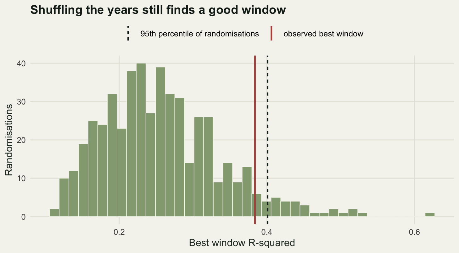
The histogram is the object the naive test pretends does not exist. Shuffling a response that genuinely depends on the weather, so that it cannot depend on it any more, still yields a best window explaining a quarter of the variance on a typical draw, and 40 per cent on the best draw in twenty.
Now check that the corrected test is calibrated. Generate null datasets, run the search, run 200 randomisations inside each, and count how often the observed best beats its own 95th percentile. If the procedure is right, that count is close to five per cent.
n_cal <- 150
n_perm_cal <- 200
set.seed(4242)
cal <- t(replicate(n_cal, {
  ww <- sim_weather(n_year)
  Wm <- win_means(ww)
  yy <- rnorm(n_year)
  obs <- max(r2_all(yy, Wm))
  c(naive = pnaive(obs, n_year) < 0.05,
    corrected = obs > quantile(perm_best_r2(yy, Wm, n_perm_cal), 0.95))
}))
print(round(c(calibration_replicates = n_cal, permutations_each = n_perm_cal,
              nominal_level = 0.05,
              naive_rate = mean(cal[, 1]), corrected_rate = mean(cal[, 2])), 4))
calibration_replicates permutations_each nominal_level
150.00 200.00 0.05
naive_rate corrected_rate
1.00 0.06 Over 150 null datasets the randomisation test rejects in 0.06 of them, against a nominal 0.05, and the naive test rejects in 1.00 of them. The correction works, and it costs one line of code that reruns a search you have already written.
rates <- data.frame(
  test = factor(c("Naive test on the\nselected window", "Randomisation test\non the whole search"),
                levels = c("Naive test on the\nselected window",
                           "Randomisation test\non the whole search")),
  rate = c(naive_fpr, mean(cal[, 2])))

ggplot(rates, aes(test, rate, fill = test)) +
  geom_col(width = 0.55) +
  geom_hline(yintercept = 0.05, colour = te_pal$ink, linetype = "22",
             linewidth = 0.6) +
  geom_text(aes(label = sprintf("%.3f", rate)), vjust = -0.6,
            colour = te_pal$ink, size = 4) +
  scale_fill_manual(values = c(te_pal$clay, te_pal$forest), guide = "none") +
  coord_cartesian(ylim = c(0, 1.08)) +
  labs(x = NULL, y = "Proportion of null datasets declared significant",
       title = "One search, two very different false positive rates") +
  theme_te()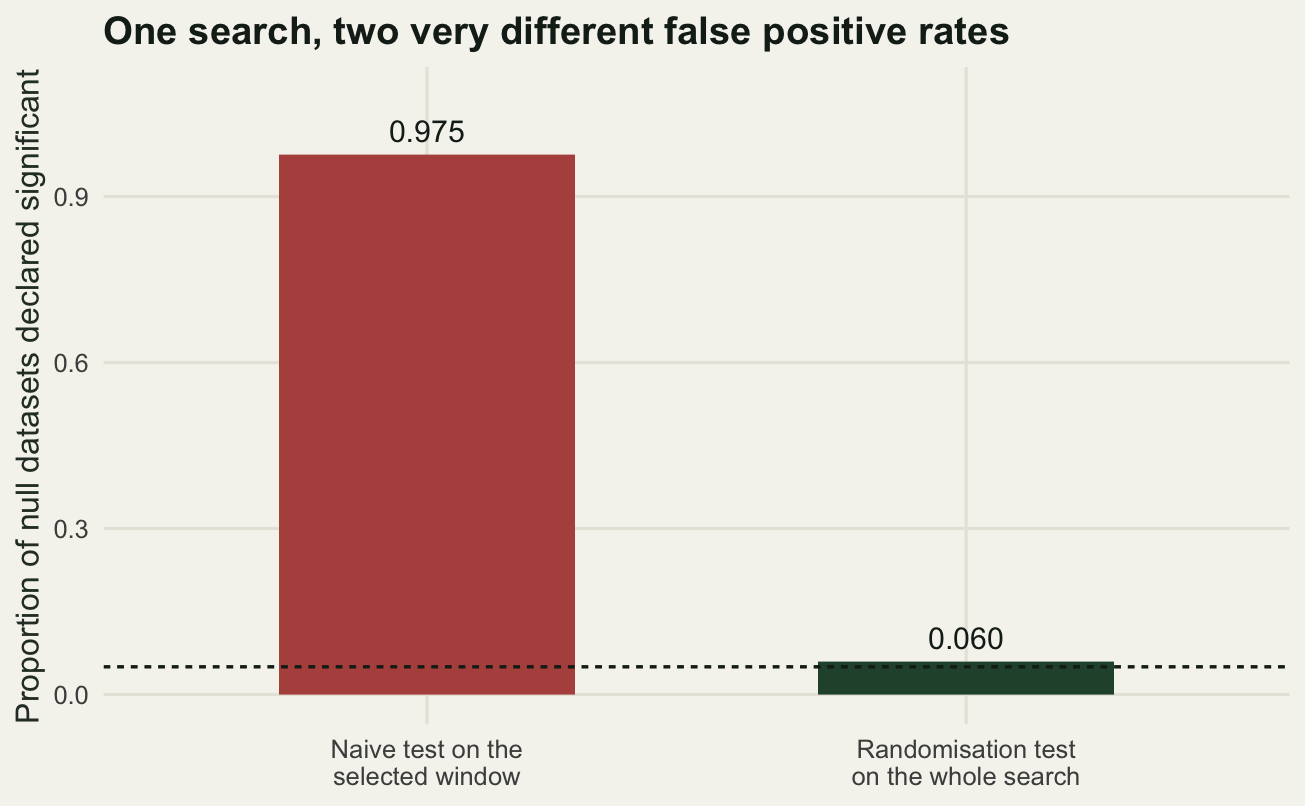
How many tests were really run
The nominal count is 4751, and a Bonferroni correction would divide the level by that number. That would be far too harsh, because neighbouring windows are not separate experiments. Two windows that differ by two days in their start share all but two of their days, and the weather inside them is autocorrelated on top of that.
The randomisation distribution already contains the answer, so no extra assumption is needed. Under \(m\) independent tests the smallest p-value has median \(1 - 0.5^{1/m}\), so inverting that for the observed median smallest p-value gives an effective count. The estimator is checked against a case where the answer is known: replace the window means with 4751 columns of independent random numbers, and it should return roughly 4751.
med_minp <- median(pnaive(pb, n_year))
m_eff <- log(0.5) / log1p(-med_minp)

set.seed(616)
V <- matrix(rnorm(n_year * n_win), n_year, n_win)
pv <- perm_best_r2(y_sig, V, n_perm)
med_minp_ind <- median(pnaive(pv, n_year))
m_eff_ind <- log(0.5) / log1p(-med_minp_ind)
m_eff_alpha <- log1p(-naive_fpr) / log1p(-0.05)

print(round(c(nominal_tests = n_win, median_min_p = med_minp,
              effective_tests = m_eff, ratio = n_win / m_eff,
              control_median_min_p = med_minp_ind,
              control_effective = m_eff_ind,
              control_recovery = m_eff_ind / n_win,
              effective_from_alpha = m_eff_alpha,
              ratio_from_alpha = n_win / m_eff_alpha), 4))
nominal_tests median_min_p effective_tests
4751.0000 0.0051 134.8489
ratio control_median_min_p control_effective
35.2320 0.0001 4639.6957
control_recovery effective_from_alpha ratio_from_alpha
0.9766 71.9174 66.0619 On independent columns the estimator returns 4639.6957 against a true 4751, so it recovers 0.9766 of the nominal count and can be trusted to within a few per cent. On the real window grid the median smallest p-value is 0.0051, which corresponds to 134.8489 effectively independent tests. The nominal count overstates the number of tests by a factor of 35.232.
There is a caveat, and it is the more interesting half of the result. The effective count is not one number: it depends on which part of the distribution you match it to. Matching the median smallest p-value gives 134.8489. Matching instead the rate at which the naive test fires, 0.975, gives 71.9174 and a ratio of 66.0619. A set of correlated tests does not behave like any single number of independent ones, so an effective count is a summary of one feature of the null distribution rather than a property of the grid. That is a reason to use the randomisation distribution directly and treat the effective count as description rather than as a correction to apply.
Either way the practical message is the same. Bonferroni at 4751 would demand a per window p-value of about one in a hundred thousand, which 30 years of data cannot deliver for any effect an ecologist would call real, so the analysis that takes the nominal count seriously simply never detects anything. The randomisation threshold sits between the two.
Where the window is, when there really is one
Suppose the effect is real and the corrected test does reject. You now report a window. How well is it located? Repeat the search over 200 replicate datasets at the same effect size, at five record lengths, and record the start and end of the selected window each time. Count a window as recovered if it overlaps the true one by more than half, measured as the shared days divided by the days covered by either.
n_rl <- 200
rl_years <- c(15, 30, 60, 90, 120)
set.seed(808)
rl <- do.call(rbind, lapply(rl_years, function(ny) {
  out <- t(replicate(n_rl, {
    ww <- sim_weather(ny)
    Wm <- win_means(ww)
    yy <- make_y(ww)
    bb <- which.max(r2_all(yy, Wm))
    s <- grid$start[bb]; e <- grid$end[bb]
    inter <- max(0, min(e, true_end) - max(s, true_start) + 1)
    unio <- max(e, true_end) - min(s, true_start) + 1
    c(start = s, end = e, iou = inter / unio, r2 = max(r2_all(yy, Wm)))
  }))
  data.frame(years = ny, sd_start = sd(out[, "start"]), sd_end = sd(out[, "end"]),
             early_start = true_start - mean(out[, "start"]),
             early_end = true_end - mean(out[, "end"]),
             mean_start = mean(out[, "start"]), mean_end = mean(out[, "end"]),
             good = mean(out[, "iou"] > 0.5), med_r2 = median(out[, "r2"]))
}))
print(c(replicates_per_length = n_rl, record_lengths = length(rl_years)))
replicates_per_length record_lengths
200 5 print(round(rl, 3)) years sd_start sd_end early_start early_end mean_start mean_end good med_r2
1 15 73.520 73.630 29.70 33.100 211.30 251.900 0.420 0.592
2 30 47.175 51.956 12.45 11.850 228.55 273.150 0.655 0.441
3 60 14.013 10.734 2.43 -1.445 238.57 286.445 0.930 0.389
4 90 5.786 7.222 0.17 -0.605 240.83 285.605 0.975 0.380
5 120 4.602 5.479 -0.06 -0.285 241.06 285.285 1.000 0.361At 15 years the standard deviation of the recovered start is 73.52 days and of the recovered end 73.63 days. The window is not located at all: the answer is a random stretch of the year, and only 0.42 of replicates overlap the truth by more than half. The means are also pulled inward, 29.7 days early at the start and 33.1 days early at the end, because a search that is mostly finding noise finds it in the middle of the grid where the most candidate windows are.
At 30 years, the length of our main dataset, the standard deviation of the start is 47.175 days. That is one and a half months. The bias has shrunk without going away, 12.45 days early at the start, and 0.655 of replicates overlap the truth. A paper reporting a 45 day spring window from 30 years of data, with the days named to the calendar, is reporting one draw from a distribution that wide.
At 60 years the standard deviation of the start falls to 14.013 days and 0.93 of replicates overlap the truth. At 90 years it is 5.786 days. At 120 years it is 4.602 days and 1.000 of replicates overlap the truth.
The last column prices the other cost. The true window explains 35 per cent of the variance. The median best window R-squared is 0.592 at 15 years, 0.441 at 30, 0.389 at 60, 0.38 at 90 and 0.361 at 120. The selected effect size is inflated at every record length in this sweep, and badly inflated at the short ones, because the winner of a search is the candidate whose noise happened to help most. If you use the fitted R-squared of the selected window to plan the next study, or to compare populations, you are propagating that inflation.
edges <- rbind(
  data.frame(years = rl$years, mid = rl$mean_start, sdv = rl$sd_start,
             edge = "Window start"),
  data.frame(years = rl$years, mid = rl$mean_end, sdv = rl$sd_end,
             edge = "Window end"))
truth_lines <- data.frame(yv = c(true_start, true_end),
                          edge = c("Window start", "Window end"))

ggplot(edges, aes(factor(years), mid, colour = edge)) +
  geom_hline(data = truth_lines, aes(yintercept = yv, colour = edge),
             linetype = "22", linewidth = 0.6) +
  geom_pointrange(aes(ymin = mid - sdv, ymax = mid + sdv),
                  position = position_dodge(width = 0.4), size = 0.6) +
  scale_colour_manual(values = c("Window start" = te_pal$forest,
                                 "Window end" = te_pal$clay), name = NULL) +
  labs(x = "Years of data", y = "Day of the record",
       title = "The window comes into focus slowly") +
  theme_te() +
  theme(legend.position = "top")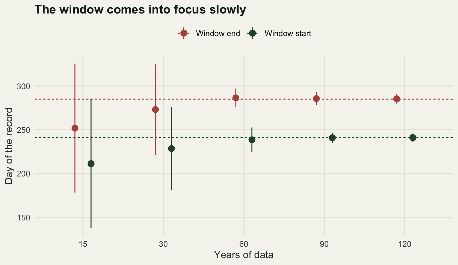
A window is not a mechanism
Everything above is about whether a window is real. Suppose it is: the corrected test rejects, the record is long, the window is located to a fortnight. What have you learnt?
You have learnt that the yearly response covaries with the mean temperature of those days. You have not learnt that temperature over those days acts on the organism. Build a case where it does not. The response is driven by a food supply index, which is itself driven by spring temperature. The weather has no path to the response except through the food. The path coefficients are set so that the correlation between the response and the true window temperature is identical to the direct case.
Two comparisons run below, not one. The first is direct effect against confound. The second is direct effect against a second, independent run of the direct effect itself, which supplies the scale on which any difference in the first comparison has to be read.
n_cf <- 400
n_pw <- 150
n_perm_cf <- 150
a_path <- rho2^0.25

draw_case <- function(ny, kind) {
  ww <- sim_weather(ny)
  wt <- as.vector(scale(rowMeans(ww[, true_start:true_end, drop = FALSE])))
  if (kind == "direct") {
    yy <- sqrt(rho2) * wt + sqrt(1 - rho2) * rnorm(ny)
    zz <- rnorm(ny)
  } else {
    zz <- a_path * wt + sqrt(1 - a_path^2) * rnorm(ny)
    yy <- a_path * zz + sqrt(1 - a_path^2) * rnorm(ny)
  }
  list(W = win_means(ww), y = yy, z = zz)
}

summarise_case <- function(d) {
  r2v <- r2_all(d$y, d$W)
  bb <- which.max(r2v)
  s <- grid$start[bb]; e <- grid$end[bb]
  inter <- max(0, min(e, true_end) - max(s, true_start) + 1)
  unio <- max(e, true_end) - min(s, true_start) + 1
  fit <- lm(d$y ~ d$W[, bb])
  c(start = s, end = e, r2 = r2v[bb], iou = inter / unio,
    shapiro = shapiro.test(residuals(fit))$p.value, cor_yz = cor(d$y, d$z))
}

set.seed(2211)
cf_d <- t(replicate(n_cf, summarise_case(draw_case(n_year, "direct"))))
set.seed(2211)
cf_c <- t(replicate(n_cf, summarise_case(draw_case(n_year, "confound"))))
set.seed(5150)
cf_d2 <- t(replicate(n_cf, summarise_case(draw_case(n_year, "direct"))))

pass_rate <- function(kind, seed) {
  set.seed(seed)
  mean(replicate(n_pw, {
    d <- draw_case(n_year, kind)
    obs <- max(r2_all(d$y, d$W))
    obs > quantile(perm_best_r2(d$y, d$W, n_perm_cf), 0.95)
  }))
}
pow_d <- pass_rate("direct", 77)
pow_c <- pass_rate("confound", 77)

arm_row <- function(m, pw) c(mean_R2 = mean(m[, "r2"]), mean_start = mean(m[, "start"]),
                            sd_start = sd(m[, "start"]), sd_end = sd(m[, "end"]),
                            recovered = mean(m[, "iou"] > 0.5), passes = pw,
                            resid_normal = mean(m[, "shapiro"] > 0.05))
print(round(rbind(direct = arm_row(cf_d, pow_d),
                  confounded = arm_row(cf_c, pow_c),
                  direct_rerun = arm_row(cf_d2, NA)), 4))
mean_R2 mean_start sd_start sd_end recovered passes resid_normal
direct 0.4364 230.580 43.0033 43.1210 0.6550 0.6200 0.9500
confounded 0.4414 231.985 42.7646 42.7814 0.6575 0.6267 0.9550
direct_rerun 0.4474 233.640 39.5459 40.8005 0.6725 NA 0.9525print(round(c(replicates_each = n_cf, power_replicates = n_pw,
path_coefficient = a_path, implied_cor_y_w = a_path^2,
confounded_cor_y_z = mean(cf_c[, "cor_yz"]),
direct_cor_y_z = mean(cf_d[, "cor_yz"]),
R2_p_confound = t.test(cf_d[, "r2"], cf_c[, "r2"])$p.value,
R2_p_rerun = t.test(cf_d[, "r2"], cf_d2[, "r2"])$p.value,
start_p_confound = t.test(cf_d[, "start"], cf_c[, "start"])$p.value,
start_p_rerun = t.test(cf_d[, "start"], cf_d2[, "start"])$p.value), 4)) replicates_each power_replicates path_coefficient implied_cor_y_w
400.0000 150.0000 0.7692 0.5916
confounded_cor_y_z direct_cor_y_z R2_p_confound R2_p_rerun
0.7605 -0.0017 0.5209 0.1539
start_p_confound start_p_rerun
0.6433 0.2952 Each path coefficient is 0.7692, so the response correlates 0.7605 with the food index in the confounded case and 0.5916 with the true window temperature, which is the same correlation the direct case has by construction. The measured summaries line up across the three arms. Mean best window R-squared is 0.4364 for the direct effect and 0.4414 for the confound. The share of replicates recovering the true window is 0.655 and 0.6575. The share passing the randomisation test is 0.62 and 0.6267. The share whose residuals pass a Shapiro test is 0.95 and 0.955. The standard deviation of the recovered start is 43.0033 days and 42.7646 days.
Read those against the calibration arm. The direct effect compared with a second independent run of itself gives a p-value of 0.1539 on mean R-squared and 0.2952 on mean recovered start. The direct effect compared with the confound gives 0.5209 and 0.6433. On this run the two mechanisms differ from each other by less than one mechanism differs from a rerun of itself.
That is not an accident of Monte Carlo error, and the algebra says why. Write out the confounded response: it is the path coefficient squared times the standardised window temperature, plus a noise term independent of the weather. The path coefficient squared is 0.5916, and the noise standard deviation is 0.8062, which are exactly the slope and the noise of the direct case. The two generating processes produce responses with identical distributions.
set.seed(96)
wt1 <- as.vector(scale(rowMeans(sim_weather(n_year)[, true_start:true_end])))
e1 <- rnorm(n_year); e2 <- rnorm(n_year)
z1 <- a_path * wt1 + sqrt(1 - a_path^2) * e1
y_conf <- a_path * z1 + sqrt(1 - a_path^2) * e2
y_dir <- sqrt(rho2) * wt1 + (a_path * sqrt(1 - a_path^2) * e1 +
                               sqrt(1 - a_path^2) * e2)
print(round(c(identical_to_1e_12 = as.numeric(max(abs(y_conf - y_dir)) < 1e-12),
              direct_slope = sqrt(rho2), confounded_slope = a_path^2,
              noise_sd_direct = sqrt(1 - rho2),
              noise_sd_confounded = sqrt(a_path^2 * (1 - a_path^2) +
                                           1 - a_path^2)), 4))
identical_to_1e_12 direct_slope confounded_slope noise_sd_direct
1.0000 0.5916 0.5916 0.8062
noise_sd_confounded
0.8062 Given the same weather and the same two noise draws, the confounded response and the direct response are the same vector: both slopes are 0.5916, both noise standard deviations are 0.8062, and the check that the two responses agree to machine precision returns 1. The dataset is not merely hard to classify. It is the same dataset. No diagnostic run on the response and the weather can tell you which story generated it, because both stories generated it.
This is the honest limit of the method, and it is not a limit that a better test fixes. The randomisation correction turns a false positive machine into a calibrated test of association. It says nothing at all about whether the association is causal, and in a climate window analysis the candidate confounds are numerous and correlated with everything: food phenology, snow cover, day length interacting with temperature, and the other weather variables you did not search. A window that survives randomisation is a licence to design an experiment, not a mechanism.
Where to go next
Two things make a window analysis worth trusting. The first is the correction measured above, which is cheap. The second is out of sample behaviour: does the window found in the first half of the record still predict the second half? That question has the same structure as the leakage problem in any tuned model, and data leakage in ecological model validation sets out how a selection step contaminates a validation split when the split comes after the selection rather than before it. The companion post to this one runs the checks on a fitted window analysis directly, including the split half test and the sensitivity of the answer to the grid you happened to search.
References
van de Pol M, Bailey LD, McLean N, Rijsdijk L, Lawson CR, Brouwer L 2016 Methods in Ecology and Evolution 7(10):1246-1257 (10.1111/2041-210X.12590)
Bailey LD, van de Pol M 2016 PLoS ONE 11(12):e0167980 (10.1371/journal.pone.0167980)
Simmons JP, Nelson LD, Simonsohn U 2011 Psychological Science 22(11):1359-1366 (10.1177/0956797611417632)
Brommer JE, Rattiste K, Wilson AJ 2008 Proceedings of the Royal Society B 275(1635):687-693 (10.1098/rspb.2007.0951)
Burnham KP, Anderson DR 2002 Model Selection and Multimodel Inference: A Practical Information-Theoretic Approach. Springer, ISBN 978-0-387-95364-9