---
title: "The scale of effect in landscape data"
description: "Fitting the same model at many buffer radii always returns a best one. The search inflates the error rate, and the landscape's grain limits how well it works."
date: "2026-08-12 13:00"
date-modified: "2026-10-14"
categories: [R, terra, spatial, landscape ecology, model selection, ecology tutorial]
image: thumbnail.png
image-alt: "A binary map of forest patches and open ground, with a regular grid of survey points that stops short of the map edges, and two concentric buffer circles of very different size around one of them."
---
*Corrected 14 October 2026: the post said a four hundred metre buffer shares most of its area with a six hundred metre one, though it covers less than half of the larger circle, and now says only that it lies wholly inside it; the paragraph on the edge bias now places the na.rm setting in the focal sum that builds the cover layers, not in the extraction. The lower bound on the correlations of neighbouring radii is now rounded down, since rounding to the nearest value could put it above the weakest pair, and adjacent radii are now called mostly, rather than all, near-copies of one another.*
*Corrected 7 October 2026: the number of survey points terra draws differs between installations, and with it which of the two radii at the bottom of the single search's profile wins, so the sentence naming the winner and the alt text of the profile figure no longer assume that the generating radius wins. The alt text of the selection figure no longer says the null puts its tallest bars at both ends, the boundary test now sets the gain of the new end candidate against that of an interior one, and the coarse-map explanation now cites the correlations either side of the generating radius instead of the weakest pair.*
*Corrected 27 September 2026: the post said the generating radius was 0.00 AIC units behind the winner, which compared the winner with itself; it now says the winner is the generating radius and the runner-up at 600 metres is 1.67 AIC units behind. The alt text of the delta AIC figure was also corrected to match the plotted values.*
Habitat does not act at a point. A bird responds to how much woodland lies within some distance of the nest, and nobody knows what that distance is, so the usual move is to measure cover in buffers of many radii, fit the same model to each, and let a criterion pick. The radius that wins is then reported as the scale of effect, sometimes as a finding in its own right.
Two things are true about that procedure. It works, in the sense that the winning radius is usually near the right one when there is a right one. And it is a search, so the number that comes out of it carries uncertainty that none of the usual output reports, and the model at the winning radius carries an error rate that is not the one on the page.
## A landscape and a set of survey points
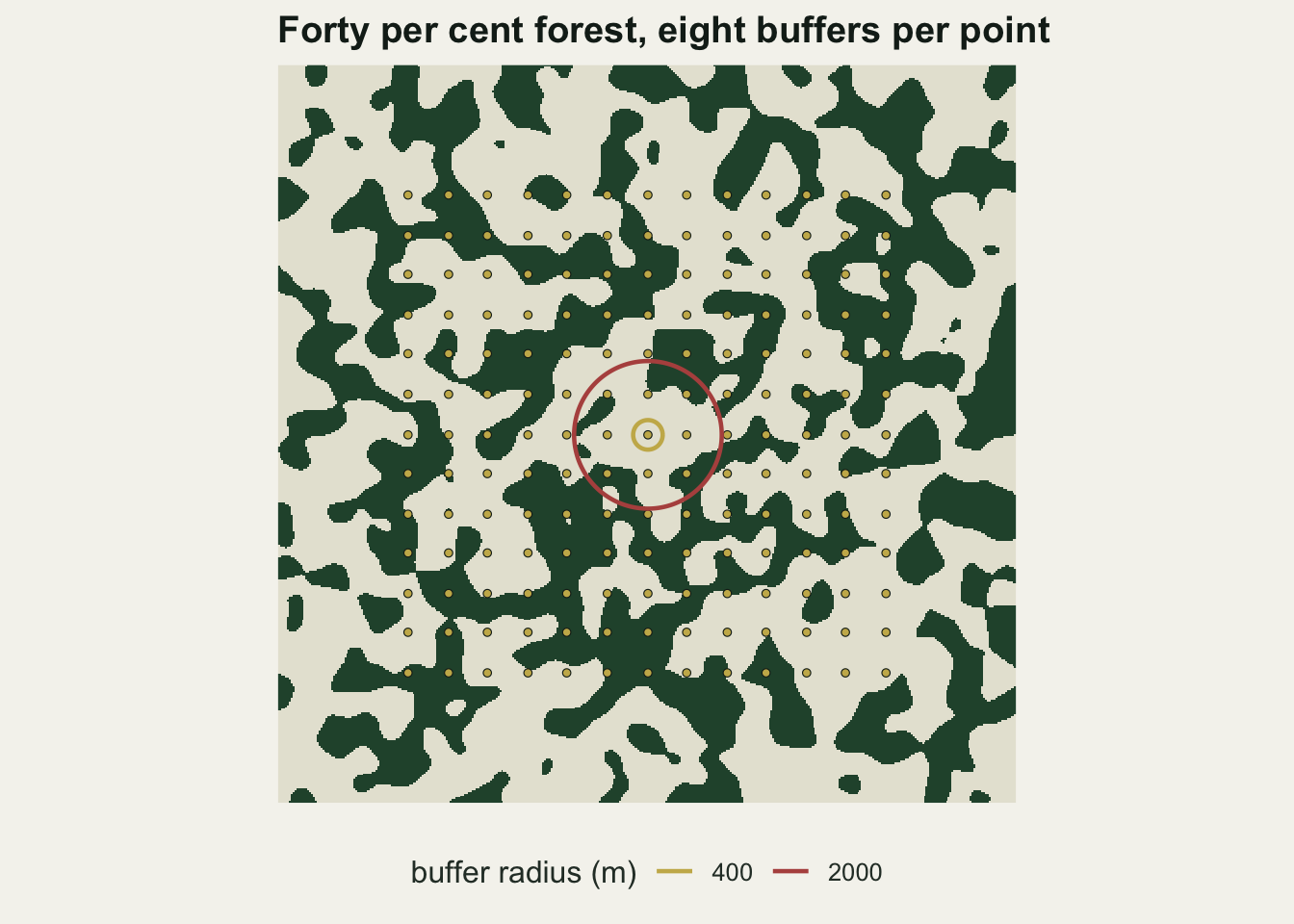
The landscape is binary, forest or open, generated so that it has spatial structure rather than being a random scatter of cells. The structure matters later, so it is a parameter from the start.
```{r setup}
#| message: false
#| warning: false
library(terra)
library(ggplot2)

te_paper  <- "#f5f4ee"
te_ink    <- "#16241d"
te_body   <- "#2c3a31"
te_forest <- "#275139"
te_rust   <- "#b5534e"
te_gold   <- "#c9b458"
te_line   <- "#dad9ca"

theme_datasheet <- function() {
  theme_minimal(base_size = 12) +
    theme(plot.background  = element_rect(fill = te_paper, colour = NA),
          panel.background = element_rect(fill = te_paper, colour = NA),
          panel.grid.major = element_line(colour = te_line, linewidth = 0.3),
          panel.grid.minor = element_blank(),
          text             = element_text(colour = te_body),
          plot.title       = element_text(colour = te_ink, face = "bold"),
          axis.text        = element_text(colour = te_body))
}

# a binary habitat map: smoothed noise, cut at a quantile to fix the cover
make_landscape <- function(range_cells, cover = 0.4, n = 400, res_m = 50) {
  r <- rast(xmin = 0, xmax = n * res_m, ymin = 0, ymax = n * res_m,
            resolution = res_m, crs = "EPSG:32634")
  values(r) <- rnorm(ncell(r))
  sm <- focal(r, focalMat(r, range_cells * res_m, "Gauss"), fun = sum,
              na.policy = "all", fillvalue = 0)
  cut_at <- global(sm, function(v, ...) quantile(v, 1 - cover, na.rm = TRUE))[1, 1]
  out <- sm > cut_at
  names(out) <- "forest"
  out
}

# proportion of forest within a circle, computed once for the whole map.
# na.rm = FALSE matters: with na.rm = TRUE a cell near the edge would be given
# the sum of a truncated circle instead of NA, which is a downward bias, not a
# missing value, and nothing downstream would notice.
cover_at <- function(land, radius_m) {
  f <- focal(land, focalMat(land, radius_m, "circle"), fun = sum,
             na.rm = FALSE, fillvalue = NA)
  names(f) <- paste0("r", radius_m)
  f
}

set.seed(20260812)
radii <- c(200, 400, 600, 800, 1000, 1400, 2000, 3000)
land  <- make_landscape(range_cells = 6)
cover <- rast(lapply(radii, function(rr) cover_at(land, rr)))

# the survey frame is inset by the widest radius, so every point has a
# complete buffer at every candidate scale
frame <- crop(land, ext(3000, 17000, 3000, 17000))
set.seed(4)
pts <- spatSample(frame, 150, "regular", as.points = TRUE, na.rm = TRUE)
X   <- terra::extract(cover, pts, ID = FALSE)
Z   <- scale(as.matrix(X))
c(points = nrow(Z), all_buffers_complete = all(complete.cases(X)))
```
That inset is the first cost of a wide search, and it is charged before any model is fitted: the widest radius decides where you are allowed to put a survey point, so a 20 kilometre map yields a 14 kilometre frame. The alternative is worse than it looks. Setting `na.rm = TRUE` in the focal sum that builds the cover layers returns a number for every cell, including the ones whose circle runs off the map, and that number is the sum of whatever part of the circle survived. It is a downward bias that grows towards the edge, it has no missing values to warn anyone, and it puts a deterministic function of position into the covariate that the widest buffers are supposed to measure.
```{r fig-landscape}
#| fig-cap: "The simulated landscape, the survey frame inset from the edge, and two of the eight buffers drawn around one point."
#| fig-alt: "A square map twenty kilometres across, dark forest patches on a pale background. A regular grid of small pale-gold survey points covers the middle of it and stops short of the edges by a clear margin on all four sides. Two circles are drawn around one point near the centre: a large one and a much smaller one a few times the width of the point."
land_df <- as.data.frame(land, xy = TRUE)
pt_df   <- as.data.frame(crds(pts))
names(pt_df) <- c("x", "y")
focus   <- pt_df[which.min((pt_df$x - 10000)^2 + (pt_df$y - 10000)^2), ]
ring    <- do.call(rbind, lapply(c(400, 2000), function(rr) {
  th <- seq(0, 2 * pi, length.out = 200)
  data.frame(x = focus$x + rr * cos(th), y = focus$y + rr * sin(th),
             radius = factor(rr))
}))

ggplot(land_df, aes(x = x, y = y)) +
  geom_raster(aes(fill = forest)) +
  geom_point(data = pt_df, shape = 21, fill = te_gold, colour = te_ink,
             size = 1.3, stroke = 0.3) +
  geom_path(data = ring, aes(group = radius, colour = radius), linewidth = 0.8) +
  scale_fill_manual(values = c(`FALSE` = "#e6e4d6", `TRUE` = te_forest)) +
  scale_colour_manual(values = c(`400` = te_gold, `2000` = te_rust)) +
  coord_equal(expand = FALSE) +
  labs(x = NULL, y = NULL, colour = "buffer radius (m)",
       title = "Forty per cent forest, eight buffers per point") +
  theme_datasheet() +
  theme(legend.position = "bottom", axis.text = element_blank(),
        panel.grid.major = element_blank()) +
  guides(fill = "none")
```
## The covariates are almost the same variable
Before any model is fitted, look at what the eight candidate predictors actually are. A 400 metre buffer lies wholly inside a 600 metre buffer, so every cell the smaller one counts is counted again by the larger one, and on a landscape whose patches are much larger than the smallest buffer the two share most of their variation.
```{r correlations}
round(cor(Z)[, c("r200", "r800", "r3000")], 2)
```
Neighbouring radii correlate above `r sprintf("%.2f", floor(100 * min(sapply(1:7, function(k) cor(Z[, k], Z[, k + 1])))) / 100)` all the way along the sequence. A model selection exercise among eight predictors that resemble each other this closely is not choosing between eight distinct hypotheses. Most adjacent radii are near-copies of one another, so whatever separates them in a given data set is small, and much of it is noise.
## The search, run once
Generate counts that really do depend on cover, at a radius of 800 metres.
```{r one-search}
true_j    <- which(radii == 800)
beta_true <- 0.2

set.seed(77)
y <- rpois(nrow(Z), exp(1.6 + beta_true * Z[, true_j]))

aic <- vapply(seq_along(radii),
              function(j) AIC(glm(y ~ Z[, j], family = poisson)), numeric(1))
data.frame(radius_m = radii, delta_aic = round(aic - min(aic), 2))
```
The effect size is `r beta_true` on the log scale per standard deviation of cover, which is respectable rather than overwhelming.
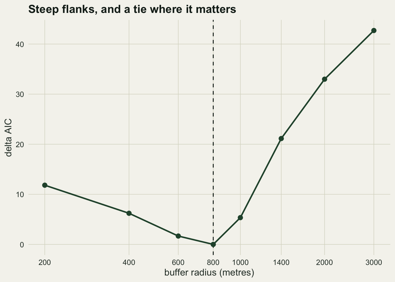
The winner is `r radii[which.min(aic)]` metres, `r if (which.min(aic) == true_j) "the radius the counts were actually generated from" else "not the radius the counts were generated from"`, and the runner-up at `r radii[order(aic)[2]]` metres is only `r sprintf("%.2f", sort(aic - min(aic))[2])` AIC units behind it, which is inside the range where two models are usually called indistinguishable. The profile is steep on both flanks and level exactly where it should not be: across the pair of radii the search has to choose between.
```{r fig-profile}
#| fig-cap: "Delta AIC against buffer radius for the single data set above. The dashed line marks the radius the counts were generated from."
#| fig-alt: "A line of eight points against buffer radius on a logarithmic axis. It falls from above ten at two hundred metres to a near-flat bottom at six hundred and eight hundred, where one point is at zero and the other within two units of it, then climbs steeply to above thirty at three thousand. A vertical dashed line at eight hundred metres passes through that flat bottom."
prof <- data.frame(radius = radii, delta = aic - min(aic))

ggplot(prof, aes(x = radius, y = delta)) +
  geom_vline(xintercept = 800, linetype = "dashed", colour = te_ink) +
  geom_line(colour = te_forest, linewidth = 0.9) +
  geom_point(colour = te_forest, size = 2.4) +
  scale_x_log10(breaks = radii) +
  labs(x = "buffer radius (metres)", y = "delta AIC",
       title = "Steep flanks, and a tie where it matters") +
  theme_datasheet()
```
## The search, run three hundred times
One data set says nothing about a procedure. Repeat the whole search over fresh counts from the same landscape and the same points, and look at the distribution of the answer rather than the answer.
```{r search-fn}
search_once <- function(y, Zm) {
  a <- vapply(seq_along(radii),
              function(j) AIC(glm(y ~ Zm[, j], family = poisson)), numeric(1))
  j <- which.min(a)
  m <- glm(y ~ Zm[, j], family = poisson)
  c(radius = radii[j], p = coef(summary(m))[2, 4],
    daic = sort(a)[2] - sort(a)[1])
}
sim <- function(beta, Zm, truth_j, nsim = 300) {
  as.data.frame(t(vapply(seq_len(nsim), function(i) {
    search_once(rpois(nrow(Zm), exp(1.6 + beta * Zm[, truth_j])), Zm)
  }, numeric(3))))
}
```
```{r sweep-true}
set.seed(101)
found <- sim(beta = 0.2, Zm = Z, truth_j = true_j)
table(found$radius)
round(c(exactly_right   = mean(found$radius == 800),
        within_one_step = mean(found$radius %in% c(600, 800, 1000)),
        median_daic     = median(found$daic)), 3)
```
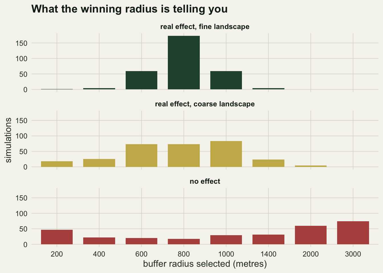
The search lands on the generating radius in `r sprintf("%.0f", 100 * mean(found$radius == 800))` per cent of runs and within one step of it in `r sprintf("%.0f", 100 * mean(found$radius %in% c(600, 800, 1000)))` per cent, which is a useful procedure. It is also a procedure whose typical margin over the runner-up is `r sprintf("%.1f", median(found$daic))` AIC units. Those two sentences describe the same experiment. The first is the one that gets written down.
## What the search does to the error rate
Now take the effect away entirely. The counts no longer depend on cover at any radius. Run the same search, and ask how often the coefficient at the winning radius comes out significant.
```{r null-effect}
set.seed(202)
null_search <- sim(beta = 0, Zm = Z, truth_j = 1)
table(null_search$radius)
mean(null_search$p < 0.05)
```
The comparison has to be against a radius fixed in advance, so take all eight in turn on the same 300 null data sets.
```{r null-fixed}
set.seed(202)
p_fixed <- t(vapply(seq_len(300), function(i) {
  y <- rpois(nrow(Z), exp(1.6))
  vapply(seq_along(radii),
         function(j) coef(summary(glm(y ~ Z[, j], family = poisson)))[2, 4],
         numeric(1))
}, numeric(length(radii))))
fixed_rate <- setNames(colMeans(p_fixed < 0.05), radii)
round(fixed_rate, 3)
```
Every radius fixed in advance behaves, near enough: the eight rates run from `r sprintf("%.2f", min(fixed_rate))` to `r sprintf("%.2f", max(fixed_rate))` around a nominal 0.05, which is the spread 300 simulations gives. Choosing the radius by AIC first takes the rate to `r sprintf("%.2f", mean(null_search$p < 0.05))`. The p value printed beside the winning coefficient is computed as though that radius had been specified before the data were seen, and it was not.
## Where the winning radius lands when there is nothing to find
The distribution of the winning radius under the null is worth a section of its own, because it is not uniform: it piles up at the two ends of the range searched. One explanation can be dismissed straight away. It is not that the extreme radii have more freedom to fit noise: every candidate here is a single predictor with a single degree of freedom, and none of them can fit more than any other.
What is left is a property of taking a minimum over a set whose members are mostly near-copies of their neighbours. Two adjacent radii usually differ by very little, so a near-tie between them is settled by noise, and an interior candidate has two close neighbours to split its wins with while an end candidate has one. That account makes two predictions, and both are checkable.
```{r boundary}
null_pick <- function(Zm, cols, nsim = 300) {
  set.seed(202)
  r <- radii[cols]
  picked <- vapply(seq_len(nsim), function(i) {
    y <- rpois(nrow(Zm), exp(1.6))
    a <- vapply(cols, function(j) AIC(glm(y ~ Zm[, j], family = poisson)),
                numeric(1))
    r[which.min(a)]
  }, numeric(1))
  round(table(factor(picked, levels = r)) / nsim, 3)
}

# prediction 1: move the boundary and the pile-up moves with it
pick_full <- null_pick(Z, 1:8)
pick_mid  <- null_pick(Z, 3:6)
pick_full
pick_mid
```
```{r boundary-control}
# prediction 2: take the correlation away and the pile-up should vanish
set.seed(606)
Z_indep <- scale(matrix(rnorm(nrow(Z) * length(radii)), ncol = length(radii)))
null_pick(Z_indep, 1:8)
```
The 600 metre buffer is an interior candidate in the first table and the smallest candidate in the second, and its share of the wins goes from `r sprintf("%.3f", as.numeric(pick_full["600"]))` to `r sprintf("%.3f", as.numeric(pick_mid["600"]))` without a single number in the data changing. A candidate kept in a shorter list can never lose wins, but the interior 800 metre buffer goes only from `r sprintf("%.3f", as.numeric(pick_full["800"]))` to `r sprintf("%.3f", as.numeric(pick_mid["800"]))`. Replace the eight buffers with eight independent columns of noise and the pile-up disappears: every candidate wins about an eighth of the time, whichever end of the list it sits at.
So the pile-up needs both ingredients. It follows the edges of the candidate set, and it exists at all only because neighbouring candidates measure almost the same thing. A scale of effect that lands exactly on the smallest or the largest radius you tried is the pattern a null produces most often, and it says more about where you stopped than about the species.
## The landscape sets the resolution of the answer
The last piece is the part specific to space. The reason neighbouring radii correlate is that the landscape has structure at some grain of its own, and buffers smaller than that grain all sample the same patch. Coarsen the landscape, hold everything else fixed, and the search loses its ability to tell radii apart.
```{r coarse}
set.seed(303)
land_coarse  <- make_landscape(range_cells = 16)
cover_coarse <- rast(lapply(radii, function(rr) cover_at(land_coarse, rr)))
Xc <- terra::extract(cover_coarse, pts, ID = FALSE)
Zc <- scale(as.matrix(Xc[complete.cases(Xc), ]))

adj <- function(M) sapply(1:7, function(k) cor(M[, k], M[, k + 1]))
round(rbind(fine = adj(Z), coarse = adj(Zc)), 3)
```
```{r coarse-search}
set.seed(404)
found_coarse <- sim(beta = 0.2, Zm = Zc, truth_j = true_j)
table(found_coarse$radius)
c(fine = mean(found$radius == 800), coarse = mean(found_coarse$radius == 800))
```
Same points, same sample size, same effect size, same set of candidate radii. The share of searches that recover the generating radius falls from `r sprintf("%.2f", mean(found$radius == 800))` to `r sprintf("%.2f", mean(found_coarse$radius == 800))`, because on the coarser map the two neighbours that compete with 800 metres are even closer copies of it: they correlate with it at `r sprintf("%.3f", adj(Zc)[3])` and `r sprintf("%.3f", adj(Zc)[4])`, against `r sprintf("%.3f", adj(Z)[3])` and `r sprintf("%.3f", adj(Z)[4])` on the fine map. The scale of effect is a property of the species, but how finely you can measure it is a property of the map.
```{r fig-selected}
#| fig-cap: "Radius selected by AIC over 300 simulations, for a real effect at 800 metres on the fine landscape, the same effect on the coarse landscape, and no effect at all."
#| fig-alt: "Three stacked panels of bars over the eight candidate radii. The top panel is a tall spike at eight hundred metres with substantial bars either side at six hundred and one thousand. The middle panel is a much lower and broader mound centred on eight hundred, with bars at every radius from two hundred to two thousand. The bottom panel is lowest in the middle of the range and rises towards both ends, two hundred and three thousand metres, with the tallest bar at one of them."
sel <- rbind(
  data.frame(radius = found$radius,        case = "real effect, fine landscape"),
  data.frame(radius = found_coarse$radius, case = "real effect, coarse landscape"),
  data.frame(radius = null_search$radius,  case = "no effect"))
sel$case   <- factor(sel$case, levels = unique(sel$case))
sel$radius <- factor(sel$radius, levels = radii)

ggplot(sel, aes(x = radius, fill = case)) +
  geom_bar(width = 0.75) +
  facet_wrap(~ case, ncol = 1) +
  scale_fill_manual(values = c(te_forest, te_gold, te_rust)) +
  labs(x = "buffer radius selected (metres)", y = "simulations",
       title = "What the winning radius is telling you") +
  theme_datasheet() +
  theme(legend.position = "none",
        strip.text = element_text(colour = te_ink, face = "bold"))
```
## What to do instead of nothing
Report the profile, not the winner. A table or plot of the criterion against radius shows the reader how flat the bottom is, and costs one figure.
Get the error rate from the search rather than from the winning model. The null experiment above is eight lines and gives the rate that actually applies to the procedure you ran.
Decide the candidate set from biology before you see the response, and say what it was. A set that runs from 200 metres to 3 kilometres because those were the round numbers is a different procedure from one bounded by a known dispersal distance, and only the second one lets a reader judge whether the answer sits at an edge.
If the radius itself is the scientific question rather than a nuisance, a model that estimates it as a parameter, with a weighting kernel whose width is fitted, gives an interval instead of a winner. That is more work and it answers the question that was asked.
## Honest limits
Everything above uses one response distribution, one landscape generator and one sample size. The direction of the results is general, and the exact numbers are not: a larger sample sharpens the profile, a stronger effect sharpens it, and a candidate set of three radii instead of eight inflates the error rate less.
The error rate reported here is for the coefficient at the selected radius under an independent-points model. Survey points in a real study are spatially correlated, which inflates it further, and the two problems are separate: fixing the correlation does not fix the search, and fixing the search does not fix the correlation.
The comparison between the fine and coarse landscapes holds the number of points fixed while changing the map, so the coarse case also has fewer effectively independent buffer measurements. That is not a confound to be removed; it is the mechanism. On a coarse landscape a fixed set of points genuinely carries less information about scale than it does on a fine one.
Every distribution above is conditional on one landscape realisation and one layout of points. A second draw of either would move the numbers, and the null selection distribution in particular depends on how strongly the candidate covariates correlate, which is a property of the map.
Nothing here says buffer sweeps should not be run. They are the honest answer to a real question, and the alternative of picking one radius by convention is worse, because it hides the same uncertainty instead of measuring it.
## References
Jackson HB, Fahrig L 2015 Global Ecology and Biogeography 24(1):52-63 (10.1111/geb.12233)
Miguet P, Jackson HB, Jackson ND, Martin AE, Fahrig L 2016 Landscape Ecology 31(6):1177-1194 (10.1007/s10980-015-0314-1)
Burnham KP, Anderson DR 2002 Model Selection and Multimodel Inference, 2nd edition, Springer, ISBN 978-0-387-95364-9
## Related tutorials
- [Climate window analysis](../climate-window-analysis/)
- [Checking a climate window analysis](../checking-a-climate-window-analysis/)
- [Patch metrics and fragmentation](../patch-metrics-and-fragmentation/)
- [Distributed lag models versus the climate window](../distributed-lag-models-for-climate/)