library(ggplot2)

te_pal <- list(forest = "#275139", green = "#2f8f63", sage = "#93a87f",
               clay = "#b5534e", gold = "#cda23f", line = "#dad9ca",
               ink = "#16241d", paper = "#f5f4ee")

theme_te <- function() {
  theme_minimal(base_size = 12) +
    theme(panel.grid.minor = element_blank(),
          panel.grid.major = element_line(colour = "#e7e6dc"),
          plot.background = element_rect(fill = "#f5f4ee", colour = NA),
          panel.background = element_rect(fill = "#f5f4ee", colour = NA),
          plot.title = element_text(face = "bold", colour = te_pal$ink),
          axis.title = element_text(colour = "#2c3a31"))
}Checking a climate window analysis
R
climate
phenology
model diagnostics
ecology tutorial
ggplot2
Four checks for a climate window analysis in R: shared trends, the choice between weather variables, held-out years, and what the search grid alone is worth.
The three earlier posts in this cluster each turn a pile of daily weather into one number a model can use. Degree days and thermal time in R accumulates temperature above a base and hands back thermal time to an event. Drought indices for ecologists turns rainfall and demand into a standardised deficit on a chosen timescale. Climate window analysis in R does the most ambitious thing of the three: it searches every start date and every end date in a season for the stretch of weather that best predicts a biological response, and lets the data choose the window. That post also measured the price. Tested against a response with no climate signal at all, the naive test declared a significant window almost every time, and the fix was a randomisation: shuffle the response across years, rerun the whole search, and compare the observed best fit against the best fit the search finds in pure noise.
This post tries to break all three, and the window search hardest. It is four checks. Each one asks a different question of the same machinery, each is a self-contained measurement against a truth we set ourselves, and each returns a number rather than an opinion. Is the window real, or are the response and the weather simply both trending? Did the search pick the right climate variable, or a correlated bystander? Does the selected window predict years it has never seen? And how much of the answer was decided by the search grid rather than by the biology?
Nothing below is quoted from a rule of thumb. Every threshold and every reference distribution is measured in the same simulator, because a number in a specification is not a measurement. The simulator is deliberately plain: daily temperature with a seasonal ramp and correlated day to day anomalies, daily rainfall built the same way, and an annual breeding output that depends on the mean temperature in one fixed window and on nothing else. The truth is known throughout, which is the only way to score a diagnostic.
The simulator, and how the search is made cheap
Each year carries 200 days of weather ending at a reference day, which is the day the response is scored: think of it as the mean fledging date of a passerine population, with the weather of the preceding spring on the shelf behind it. Daily temperature is a seasonal ramp plus an autocorrelated anomaly. Daily rainfall is built from a second autocorrelated series, exponentiated so it stays positive. The response is annual mean fledglings per pair, and it depends on the mean temperature between 88 and 62 days before the reference day, a 27 day stretch that sits nowhere in particular on the search grid.
A window search is a large number of regressions, so it pays to make each one free. The mean temperature over any window is a difference of two cumulative sums divided by a length, which is constant time once the cumulative sums exist. That turns the whole grid into one matrix, and the regression of the response on every column of that matrix is one crossproduct. The randomisation test then costs almost nothing extra, because permuting the response is another matrix, not another loop.
n_day <- 200      # days of weather stored per year
ref_day <- 180    # index of the reference day, the day the response is scored
max_lag <- 150    # furthest back any window may open
true_open <- 88
true_close <- 62
b_true <- -0.18
sd_strong <- 0.23
sd_weak <- 0.50
rho_day <- 0.75
sd_day <- 2.5
rain_mu <- 2.5
sd_lograin <- 0.8

season_temp <- function(d) 12 + 12 * d / n_day

sim_climate <- function(nyr, rho = rho_day, sd_t = sd_day, sd_lr = sd_lograin,
                        rmu = rain_mu, warm = 0, cor_tp = 0) {
  zt <- matrix(0, nyr, n_day); zp <- matrix(0, nyr, n_day)
  et <- matrix(rnorm(nyr * n_day), nyr, n_day)
  ep <- matrix(rnorm(nyr * n_day), nyr, n_day)
  zt[, 1] <- et[, 1]; zp[, 1] <- ep[, 1]
  a <- sqrt(1 - rho^2)
  for (d in 2:n_day) {
    zt[, d] <- rho * zt[, d - 1] + a * et[, d]
    zp[, d] <- rho * zp[, d - 1] + a * ep[, d]
  }
  lag_of <- ref_day - seq_len(n_day)
  w <- ifelse(lag_of >= true_close & lag_of <= true_open, cor_tp, 0)
  zpm <- sweep(zp, 2, sqrt(1 - w^2), "*") + sweep(zt, 2, w, "*")
  yc <- seq_len(nyr) - (nyr + 1) / 2
  temp <- matrix(season_temp(seq_len(n_day)), nyr, n_day, byrow = TRUE) +
    sd_t * zt + warm * yc
  list(temp = temp, rain = rmu * exp(sd_lr * zpm - sd_lr^2 / 2),
       year = seq_len(nyr))
}

true_cols <- (ref_day - true_open):(ref_day - true_close)
true_mean <- function(cl) rowMeans(cl$temp[, true_cols])

cumzero <- function(x) cbind(0, t(apply(x, 1, cumsum)))

make_grid <- function(step = 5, maxlag = max_lag, min_len = 5, max_len = Inf) {
  b <- seq(0, maxlag, by = step)
  g <- expand.grid(close = b, open = b)
  g <- g[g$open - g$close + 1 >= min_len & g$open - g$close + 1 <= max_len, ]
  g[order(g$open, g$close), ]
}

win_means <- function(cs, grid, ref = ref_day) {
  i1 <- ref - grid$open; i2 <- ref - grid$close
  sweep(cs[, i2 + 1, drop = FALSE] - cs[, i1, drop = FALSE], 2, i2 - i1 + 1, "/")
}

search_windows <- function(W, y) {
  yc <- y - mean(y)
  Wc <- sweep(W, 2, colMeans(W))
  sxy <- as.vector(crossprod(Wc, yc)); sxx <- colSums(Wc^2); syy <- sum(yc^2)
  r2 <- sxy^2 / (sxx * syy); j <- which.max(r2); n <- length(y)
  tt <- sqrt(r2[j] * (n - 2) / (1 - r2[j]))
  list(j = j, r2 = r2[j], slope = sxy[j] / sxx[j], sxx = sxx[j],
       p = 2 * pt(-abs(tt), n - 2), rss = syy * (1 - r2[j]))
}

perm_max_r2 <- function(W, y, nperm) {
  n <- length(y)
  Y <- matrix(0, n, nperm)
  for (k in seq_len(nperm)) Y[, k] <- sample(y)
  Yc <- sweep(Y, 2, colMeans(Y)); Wc <- sweep(W, 2, colMeans(W))
  r2 <- sweep(sweep(crossprod(Wc, Yc)^2, 1, colSums(Wc^2), "/"), 2, colSums(Yc^2), "/")
  apply(r2, 2, max)
}

detrend <- function(M, year) {
  X <- cbind(1, year - mean(year))
  M - X %*% solve(crossprod(X), crossprod(X, M))
}

grid5 <- make_grid(5)
set.seed(20260719)
demo <- sim_climate(2000)
round(c(days_stored = n_day, reference_day_index = ref_day, longest_lag = max_lag,
        true_window_open = true_open, true_window_close = true_close,
        true_window_length = true_open - true_close + 1,
        windows_on_default_grid = nrow(grid5),
        daily_autocorrelation = rho_day, daily_temp_sd = sd_day,
        mean_daily_rain_mm = rain_mu), 4)
days_stored reference_day_index longest_lag
200.00 180.00 150.00
true_window_open true_window_close true_window_length
88.00 62.00 27.00
windows_on_default_grid daily_autocorrelation daily_temp_sd
465.00 0.75 2.50
mean_daily_rain_mm
2.50 round(c(true_slope = b_true, strong_noise_sd = sd_strong, weak_noise_sd = sd_weak,
sd_true_window_mean = sd(true_mean(demo)),
mean_true_window_temp = mean(true_mean(demo)),
strong_true_r2 = (b_true * sd(true_mean(demo)))^2 /
((b_true * sd(true_mean(demo)))^2 + sd_strong^2),
weak_true_r2 = (b_true * sd(true_mean(demo)))^2 /
((b_true * sd(true_mean(demo)))^2 + sd_weak^2)), 4) true_slope strong_noise_sd weak_noise_sd
-0.1800 0.2300 0.5000
sd_true_window_mean mean_true_window_temp strong_true_r2
1.1971 18.2823 0.4674
weak_true_r2
0.1566 The default grid steps every 5 days out to 150, which gives 465 candidate windows. Across a long run of simulated years the mean temperature in the true window averages 18.2823 degrees with a standard deviation between years of 1.1971, so the true effect of -0.18 fledglings per pair per degree moves the response by about a fifth of a fledgling for each standard deviation of window temperature. Two levels of residual noise are used below. The strong case, with a residual standard deviation of 0.23, gives the true window an R-squared of 0.4674, which is the kind of number a well behaved laying date analysis reports. The weak case, at 0.50, gives 0.1566, which is closer to what a breeding success analysis usually gets. Some of these checks bite hardest at one end and some at the other, so both are used, and each check says which.
Check 1: is the window real, or is it a shared trend?
Nearly every long term dataset in ecology has a trend, and so does nearly every long weather series. Give the response its own downward trend for reasons that have nothing to do with temperature, give the temperature a warming trend, and connect them not at all. Then run the search. Any window whose mean temperature climbs across years will correlate with a response that falls across years, and the search will find the window that does it best.
The randomisation test from the previous post is the obvious defence, so it is included from the start. For each replicate the response is permuted across years 199 times, the whole search is rerun on each permutation, and the observed best R-squared is compared against that distribution.
n_yr1 <- 40; n_rep1 <- 200; n_perm <- 199
warm_rate <- 0.07; y_trend <- -0.035

one_c1 <- function(warm, trend_y, b, sdy) {
  cl <- sim_climate(n_yr1, warm = warm)
  yc <- cl$year - mean(cl$year)
  tw <- true_mean(cl)
  y <- 4 + trend_y * yc + b * (tw - mean(tw)) + rnorm(n_yr1, 0, sdy)
  W <- win_means(cumzero(cl$temp), grid5)
  s <- search_windows(W, y)
  pm1 <- perm_max_r2(W, y, n_perm)
  pr <- (1 + sum(pm1 >= s$r2)) / (n_perm + 1)
  Wd <- detrend(W, cl$year); yd <- as.vector(detrend(cbind(y), cl$year))
  s2 <- search_windows(Wd, yd)
  pm2 <- perm_max_r2(Wd, yd, n_perm)
  pr2 <- (1 + sum(pm2 >= s2$r2)) / (n_perm + 1)
  data.frame(r2 = s$r2, p = s$p, pr = pr, slope = s$slope,
             r2d = s2$r2, pd = s2$p, prd = pr2, slope_d = s2$slope,
             thr = as.numeric(quantile(pm1, 0.95)),
             thr_d = as.numeric(quantile(pm2, 0.95)),
             trend_var = var(warm * yc), tot_var = var(tw))
}

set.seed(101)
c1_null <- do.call(rbind, replicate(n_rep1, one_c1(warm_rate, y_trend, 0, sd_weak),
                                    simplify = FALSE))
round(c(years = n_yr1, replicates = n_rep1, permutations = n_perm,
        warming_per_year = warm_rate, total_warming = warm_rate * (n_yr1 - 1),
        response_trend_per_year = y_trend,
        median_best_r2 = median(c1_null$r2),
        null_percentile = 0.95,
        naive_p_below_05 = mean(c1_null$p < 0.05),
        randomisation_p_below_05 = mean(c1_null$pr < 0.05)), 4)
years replicates permutations
40.0000 200.0000 199.0000
warming_per_year total_warming response_trend_per_year
0.0700 2.7300 -0.0350
median_best_r2 null_percentile naive_p_below_05
0.3463 0.9500 1.0000
randomisation_p_below_05
0.8100 round(c(median_best_r2_detrended = median(c1_null$r2d),
naive_p_below_05_detrended = mean(c1_null$pd < 0.05),
randomisation_p_below_05_detrended = mean(c1_null$prd < 0.05)), 4) median_best_r2_detrended naive_p_below_05_detrended
0.1482 0.8450
randomisation_p_below_05_detrended
0.0500 Across 200 replicates of 40 years, with the temperature warming by 0.07 degrees a year and the response falling by 0.035 fledglings a year for unrelated reasons, the search finds a window with a median R-squared of 0.3463. The naive p-value is below 0.05 in every single replicate, which is what the previous post led us to expect. The randomisation test, which fixed that problem when the response was plain noise, calls the window real in 0.81 of replicates. It does not help here, and the reason is mechanical: permuting the response destroys its trend, so the permuted null is a distribution of best fits against a response with no trend, which is not the null we need.
Detrending both series first is the standard repair. Regress the response on year and keep the residuals; do the same to every column of the window matrix; then search. The median best R-squared falls to 0.1482, and the randomisation test now calls a window in 0.05 of replicates, which is exactly nominal. The naive p-value is still below 0.05 in 0.845 of replicates, because detrending never touched the multiple testing problem: those two failures are independent, and fixing one leaves the other exactly where it was.
lv1 <- c("Raw series, both trending", "Both series detrended")
d1 <- rbind(data.frame(thr = c1_null$thr, r2 = c1_null$r2, panel = lv1[1]),
            data.frame(thr = c1_null$thr_d, r2 = c1_null$r2d, panel = lv1[2]))
d1$panel <- factor(d1$panel, levels = lv1)
d1$called <- ifelse(d1$r2 > d1$thr, "window called real", "not called")

ggplot(d1, aes(thr, r2, colour = called)) +
  geom_abline(slope = 1, intercept = 0, colour = te_pal$ink, linetype = "22") +
  geom_point(size = 1.8, alpha = 0.85) +
  facet_wrap(~panel) +
  scale_colour_manual(values = c("window called real" = te_pal$clay,
                                 "not called" = te_pal$sage), name = NULL) +
  labs(x = "95th percentile of the replicate's own randomisation null",
       y = "Best window R squared",
       title = "A shared trend walks straight through the randomisation test") +
  theme_te() +
  theme(legend.position = "top",
        strip.text = element_text(colour = te_pal$ink, face = "bold"),
        plot.margin = margin(5.5, 14, 5.5, 5.5))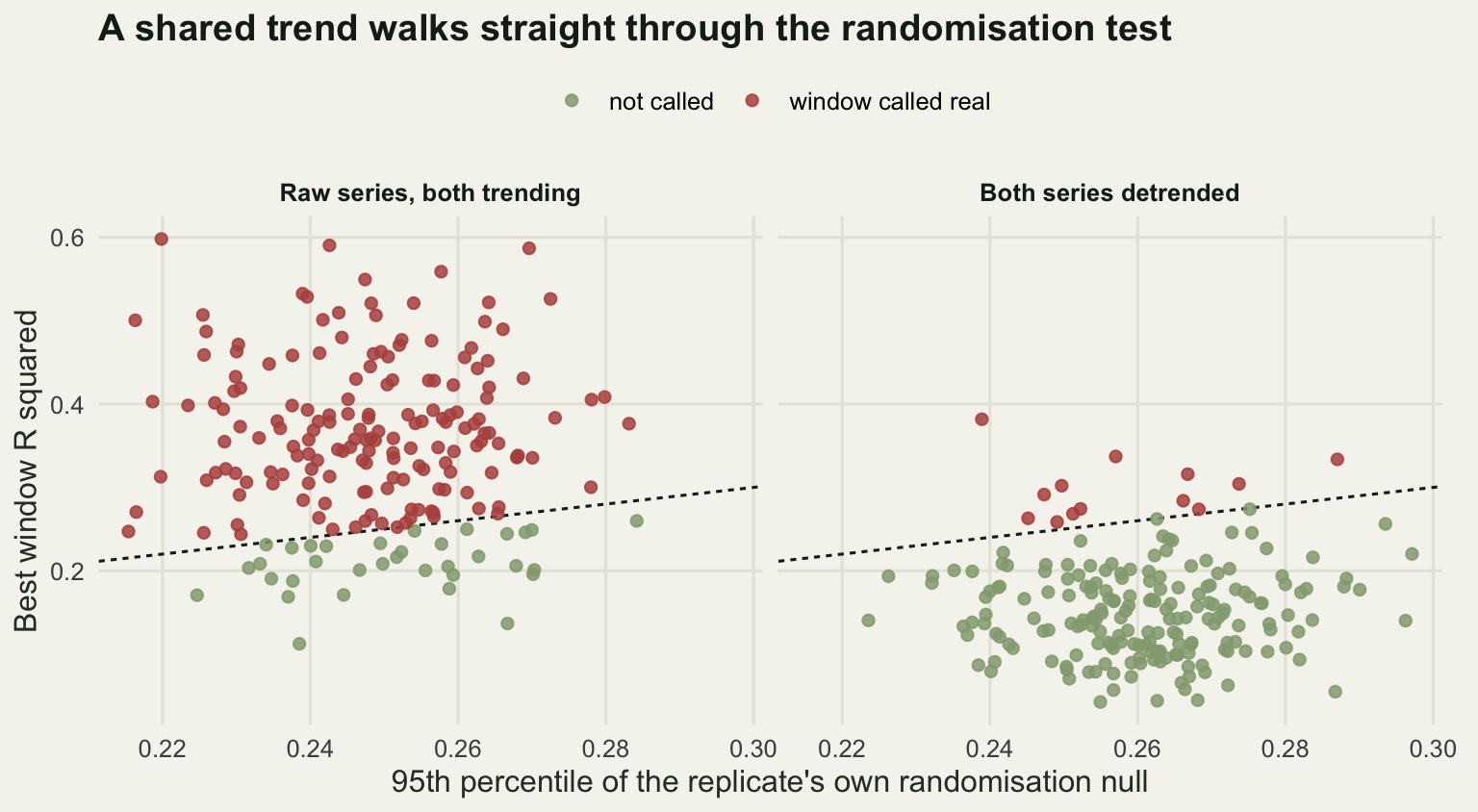
So detrend everything and move on? That is where most treatments stop, and it is where the second half of this check starts, because detrending is not free. Take a real climate signal, with the true window driving the response exactly as specified, and let the temperature warm at the same 0.07 degrees a year. Part of the effect now arrives through the trend, and detrending throws that part away before the search ever sees it.
set.seed(102)
c1_real <- do.call(rbind, replicate(n_rep1, one_c1(warm_rate, 0, b_true, sd_weak),
                                    simplify = FALSE))
round(c(driver_variance_in_trend_pct = 100 * median(c1_real$trend_var / c1_real$tot_var),
        slope_pct_of_truth = 100 * median(c1_real$slope) / b_true,
        slope_pct_of_truth_detrended = 100 * median(c1_real$slope_d) / b_true,
        slope_iqr_pct = 100 * IQR(c1_real$slope) / abs(b_true),
        slope_iqr_pct_detrended = 100 * IQR(c1_real$slope_d) / abs(b_true),
        power = mean(c1_real$pr < 0.05),
        power_detrended = mean(c1_real$prd < 0.05)), 4)
driver_variance_in_trend_pct slope_pct_of_truth
32.1809 108.1243
slope_pct_of_truth_detrended slope_iqr_pct
121.1159 61.3780
slope_iqr_pct_detrended power
97.1987 0.6300
power_detrended
0.4300 The warming accounts for 32.1809 per cent of the between year variance in the true window’s mean temperature, so detrending discards roughly a third of the driver before the search begins. What that costs is not what I expected, and the measurement is worth more than the expectation. The recovered slope is 108.1243 per cent of the truth on the raw series and 121.1159 per cent of the truth after detrending. Detrending removes none of the effect from the point estimate. It makes the point estimate slightly worse, because the selection bias that inflates a searched slope grows as the signal weakens, and detrending weakens the signal.
The price is paid in the other two currencies. The interquartile range of the estimated slope widens from 61.378 per cent of the true value to 97.1987 per cent, so the same analysis on the same biology returns an estimate whose spread is now comparable to the effect itself. And the power of the randomisation test to detect the real window falls from 0.63 to 0.43. A third of the driver’s variance bought a third of the detections.
That is the honest shape of the trade. If the response and the weather trend for separate reasons, not detrending gives a false positive rate near one and detrending brings it back to nominal, which is decisive. If the climate signal itself acts partly through the trend, detrending costs a third of your power and buys nothing back in accuracy. You cannot tell which case you are in from the data, because both produce the same picture: two trending series that correlate. What you can do is report both analyses, and treat a window that only survives on the raw series as a hypothesis rather than a result.
Check 2: which climate variable?
An analyst rarely searches one variable. Temperature and rainfall both go into the grid, and the window with the best fit wins. Set the truth so that only temperature matters, put rainfall through the identical search, and count how often rainfall wins anyway. The weak signal is used here, because that is where variable choice actually bites.
The second case is the one that matters in the field. Hot spells are dry spells, so temperature and rainfall are correlated inside the very window that drives the biology. The simulator does that by correlating the two daily anomaly series at -0.8, but only across the days of the true window, which is the cleanest way to make rainfall a proxy for temperature exactly where it hurts.
n_rep2 <- 200
one_c2 <- function(ctp, sdy, b) {
  cl <- sim_climate(n_yr1, cor_tp = ctp)
  tw <- true_mean(cl)
  y <- 4 + b * (tw - mean(tw)) + rnorm(n_yr1, 0, sdy)
  st <- search_windows(win_means(cumzero(cl$temp), grid5), y)
  sp <- search_windows(win_means(cumzero(cl$rain), grid5), y)
  data.frame(r2t = st$r2, r2p = sp$r2, daic = n_yr1 * log(sp$rss / st$rss))
}
cor_tp_hard <- -0.8
set.seed(201)
c2_indep <- do.call(rbind, replicate(n_rep2, one_c2(0, sd_weak, b_true), simplify = FALSE))
set.seed(202)
c2_corr <- do.call(rbind, replicate(n_rep2, one_c2(cor_tp_hard, sd_weak, b_true), simplify = FALSE))
set.seed(203)
c2_nosig <- do.call(rbind, replicate(n_rep2, one_c2(cor_tp_hard, sd_weak, 0), simplify = FALSE))
round(c(replicates = n_rep2, correlation_in_true_window = cor_tp_hard,
        rain_wins_independent = mean(c2_indep$r2p > c2_indep$r2t),
        rain_wins_correlated = mean(c2_corr$r2p > c2_corr$r2t),
        median_r2_temp = median(c2_corr$r2t), median_r2_rain = median(c2_corr$r2p),
        median_gap_independent = median(abs(c2_indep$daic)),
        median_gap_correlated = median(abs(c2_corr$daic))), 4)
replicates correlation_in_true_window
200.0000 -0.8000
rain_wins_independent rain_wins_correlated
0.2000 0.3050
median_r2_temp median_r2_rain
0.2300 0.1893
median_gap_independent median_gap_correlated
5.0246 3.1399 round(c(null_quantile = 0.9, median_gap_no_signal = median(abs(c2_nosig$daic)),
q90_gap_no_signal = as.numeric(quantile(abs(c2_nosig$daic), 0.9)),
share_gap_below_no_signal_q90 =
mean(abs(c2_corr$daic) <= quantile(abs(c2_nosig$daic), 0.9)),
share_gap_below_2 = mean(abs(c2_corr$daic) < 2)), 4) null_quantile median_gap_no_signal
0.9000 2.1931
q90_gap_no_signal share_gap_below_no_signal_q90
6.1402 0.7350
share_gap_below_2
0.3400 When rainfall has nothing whatever to do with the response, the best rainfall window beats the best temperature window in 0.2 of replicates. That is the baseline cost of adding a second variable to the search: a fifth of the time the analysis names a variable that did nothing at all, purely because the rainfall grid gets its own 465 chances to fit the noise in the response. Make rainfall correlated with temperature inside the true window and the rate rises to 0.305. The median best R-squared is 0.23 for temperature and 0.1893 for rainfall, so on the average replicate temperature does lead, but not by enough to survive one draw of the dice.
lv2 <- c("Rainfall unrelated to temperature", "Rainfall correlated inside the true window")
q90_gap <- as.numeric(quantile(abs(c2_nosig$daic), 0.9))
d2 <- rbind(data.frame(c2_indep, panel = lv2[1]), data.frame(c2_corr, panel = lv2[2]))
d2$panel <- factor(d2$panel, levels = lv2)
d2$gap <- ifelse(abs(d2$daic) <= q90_gap, "gap no larger than chance gives",
                 "gap beyond the chance range")

ggplot(d2, aes(r2t, r2p, colour = gap)) +
  geom_abline(slope = 1, intercept = 0, colour = te_pal$ink, linetype = "22") +
  geom_point(size = 1.8, alpha = 0.85) +
  facet_wrap(~panel) +
  scale_colour_manual(values = c("gap no larger than chance gives" = te_pal$clay,
                                 "gap beyond the chance range" = te_pal$forest), name = NULL) +
  labs(x = "Best temperature window R squared", y = "Best rainfall window R squared",
       title = "The wrong variable wins often enough to matter") +
  theme_te() +
  theme(legend.position = "top",
        strip.text = element_text(colour = te_pal$ink, face = "bold"))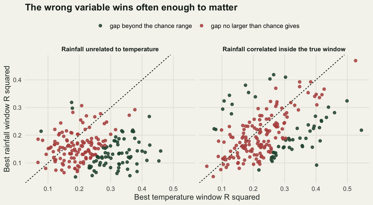
The natural next move is to price the choice with an information criterion. Both winners are simple regressions with the same number of parameters, so the AIC difference is the sample size times the log ratio of the residual sums of squares, and nothing else. In the correlated case the median gap between the two best windows is 3.1399, and 0.34 of replicates have a gap below 2.
Two on the AIC scale is a number borrowed from a setting this one does not resemble, so it is worth measuring what a meaningless gap looks like here. Run the same two searches against a response with no climate signal in it at all. Both winners are then pure selection artefacts, and the gap between them is a gap between two maxima of 465 correlated statistics. Its median is 2.1931 and its 90th percentile is 6.1402. Set the observed gaps against that distribution and 0.735 of the correlated replicates fall inside the range that chance alone produces. The gap that names the climate variable is, in three cases out of four, no bigger than the gap two unrelated searches hand you for nothing.
Check 3: does it predict out of sample?
The first two checks are about the search. This one is about the model that comes out of it. Split the years into a search set and a held-out set, run the entire selection on the search set alone, then fix the window, the slope and the intercept and score them on years the search never touched. The score is the ordinary R-squared computed against the held-out years’ own mean, so it is signed: a model that predicts worse than the held-out mean scores below zero.
Thirty search years and a held-out set from 4 to 30 years long, under a true signal and under pure noise, with the strong noise level so that the true window explains a bit under half the variance.
n_search <- 30
holds <- c(4, 6, 8, 10, 12, 15, 20, 25, 30)
n_rep3 <- 200
one_c3 <- function(b, sdy) {
  n_tot <- n_search + max(holds)
  cl <- sim_climate(n_tot); tw <- true_mean(cl)
  y <- 4 + b * (tw - mean(tw)) + rnorm(n_tot, 0, sdy)
  W <- win_means(cumzero(cl$temp), grid5); tr <- seq_len(n_search)
  s <- search_windows(W[tr, ], y[tr]); x <- W[, s$j]
  pred <- mean(y[tr]) - s$slope * mean(x[tr]) + s$slope * x
  r2h <- sapply(holds, function(h) {
    ii <- n_search + seq_len(h)
    1 - sum((y[ii] - pred[ii])^2) / sum((y[ii] - mean(y[ii]))^2)
  })
  data.frame(ins = s$r2, t(setNames(r2h, paste0("h", holds))))
}
set.seed(301)
c3_sig <- do.call(rbind, replicate(n_rep3, one_c3(b_true, sd_strong), simplify = FALSE))
set.seed(302)
c3_nul <- do.call(rbind, replicate(n_rep3, one_c3(0, sd_strong), simplify = FALSE))
set.seed(303)
c3_wk <- do.call(rbind, replicate(n_rep3, one_c3(b_true, sd_weak), simplify = FALSE))
h_ref <- 15
round(c(search_years = n_search, held_out_years = h_ref, replicates = n_rep3,
        in_sample_r2_signal = median(c3_sig$ins),
        held_out_r2_signal = median(c3_sig[[paste0("h", h_ref)]]),
        shrinkage_signal = median(c3_sig$ins) - median(c3_sig[[paste0("h", h_ref)]]),
        in_sample_r2_noise = median(c3_nul$ins),
        held_out_r2_noise = median(c3_nul[[paste0("h", h_ref)]]),
        shrinkage_noise = median(c3_nul$ins) - median(c3_nul[[paste0("h", h_ref)]])), 4)
search_years held_out_years replicates in_sample_r2_signal
30.0000 15.0000 200.0000 0.5139
held_out_r2_signal shrinkage_signal in_sample_r2_noise held_out_r2_noise
0.2951 0.2187 0.1921 -0.3020
shrinkage_noise
0.4941 pow_tab <- do.call(rbind, lapply(holds, function(h) {
cn <- paste0("h", h); thr <- as.numeric(quantile(c3_nul[[cn]], 0.95))
data.frame(held_out_years = h, noise_q95 = thr,
median_signal = median(c3_sig[[cn]]),
power_strong = mean(c3_sig[[cn]] > thr),
power_weak = mean(c3_wk[[cn]] > thr))
}))
print(round(pow_tab, 4)) held_out_years noise_q95 median_signal power_strong power_weak
1 4 0.3746 0.0182 0.285 0.115
2 6 0.2584 0.1575 0.430 0.135
3 8 0.2554 0.2472 0.485 0.135
4 10 0.1674 0.2732 0.595 0.190
5 12 0.1571 0.2695 0.620 0.155
6 15 0.0872 0.2951 0.720 0.220
7 20 0.0574 0.3302 0.790 0.265
8 25 0.0108 0.3279 0.855 0.305
9 30 0.0100 0.3147 0.875 0.330round(c(smallest_hold_80pc = min(pow_tab$held_out_years[pow_tab$power_strong >= 0.8]),
power_weak_at_30 = pow_tab$power_weak[pow_tab$held_out_years == 30],
held_out_r2_noise_at_30 = median(c3_nul$h30)), 4) smallest_hold_80pc power_weak_at_30 held_out_r2_noise_at_30
25.0000 0.3300 -0.2848 With a real signal the selected window reports a median in-sample R-squared of 0.5139 and scores 0.2951 on 15 held-out years. The shrinkage is 0.2187, which is to say that much of what the analysis reports is the search fitting itself. With no signal at all the selected window still reports 0.1921 in sample, and scores -0.302 out of sample, a shrinkage of 0.4941.
That negative number is the whole check. I expected the held-out score under noise to sit on zero and it does not: it sits below zero, and it does so for a reason worth stating. A window selected against noise comes with a slope that is not small, because the search chose it for being large. Applied to new years that slope adds variance and nothing else, so the predictions are worse than simply quoting the mean. Under noise, the model is not uninformative; it is actively harmful, and the held-out score says so with a sign.
library(grid)
lv3 <- c("In sample against held out, 15 held out years",
         "Power to tell the two cases apart")
clamp <- function(v) pmax(v, -1.5)
pa <- rbind(data.frame(x = c3_sig$ins, y = clamp(c3_sig$h15), grp = "true signal"),
            data.frame(x = c3_nul$ins, y = clamp(c3_nul$h15), grp = "pure noise"))
pa$panel <- factor(lv3[1], levels = lv3)
pb <- rbind(data.frame(x = pow_tab$held_out_years, y = pow_tab$power_strong,
                       grp = "true signal"),
            data.frame(x = pow_tab$held_out_years, y = pow_tab$power_weak,
                       grp = "weak signal"))
pb$panel <- factor(lv3[2], levels = lv3)

p_scatter <- ggplot(pa, aes(x, y, colour = grp)) +
  geom_hline(yintercept = 0, colour = te_pal$ink, linetype = "22") +
  geom_point(size = 1.7, alpha = 0.8) +
  facet_wrap(~panel) +
  scale_colour_manual(values = c("true signal" = te_pal$forest,
                                 "pure noise" = te_pal$clay), name = NULL) +
  labs(x = "In sample R squared", y = "Held out R squared") +
  theme_te() +
  theme(legend.position = "top",
        strip.text = element_text(colour = te_pal$ink, face = "bold"),
        plot.margin = margin(2, 12, 5.5, 5.5))

p_power <- ggplot(pb, aes(x, y, colour = grp)) +
  geom_hline(yintercept = 0.8, colour = te_pal$ink, linetype = "22") +
  geom_line(linewidth = 0.9) +
  geom_point(size = 2.2) +
  facet_wrap(~panel) +
  scale_colour_manual(values = c("true signal" = te_pal$forest,
                                 "weak signal" = te_pal$gold), name = NULL) +
  labs(x = "Number of held out years", y = "Power") +
  theme_te() +
  theme(legend.position = "top",
        strip.text = element_text(colour = te_pal$ink, face = "bold"),
        plot.margin = margin(2, 12, 5.5, 5.5))

grid.newpage()
grid.rect(gp = gpar(fill = te_pal$paper, col = NA))
pushViewport(viewport(layout = grid.layout(
  2, 2, heights = unit.c(unit(2, "lines"), unit(1, "null")))))
pushViewport(viewport(layout.pos.row = 1, layout.pos.col = 1:2))
grid.text("Held out years are where a selected window pays for itself",
          x = unit(6, "points"), hjust = 0,
          gp = gpar(fontface = "bold", col = te_pal$ink, cex = 1.2))
popViewport()
print(p_scatter, vp = viewport(layout.pos.row = 2, layout.pos.col = 1))
print(p_power, vp = viewport(layout.pos.row = 2, layout.pos.col = 2))
popViewport()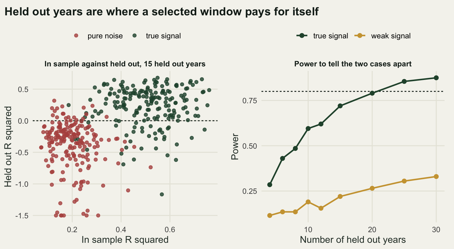
Now the practical question: how many held-out years does it take? Take the 95th percentile of the noise distribution as the threshold and count how often the signal case clears it. With four held-out years the threshold is 0.3746, which is higher than most real windows manage out of sample, and the power is 0.285. On this run the curve climbs as the threshold falls, reaching 0.72 at fifteen held-out years and 0.79 at twenty, and it first passes four fifths at 25. Against a window that genuinely explains a bit under half the variance, this check needs 25 to 30 held-out years on top of the 30 the search consumed, and where the crossing falls is an estimate from 200 replicates rather than a fixed requirement.
The weak signal never gets there at all. At thirty held-out years its power is 0.33, because a window explaining a sixth of the variance simply cannot out-predict the held-out mean often enough to stand out. That is not a failure of the check, it is the check reporting something true: with that effect size and that many years, nothing distinguishes the fitted window from a selection artefact, and no amount of care with the p-value changes it.
Read the check in the direction that is cheap, then. Reaching four fifths power to confirm a window takes more years than most studies have. Landing well below zero, where the noise case sits at a median of -0.302, needs only fifteen, and a score down there is decisive in the other direction. The check is much better at killing windows than at blessing them, which is what you want from a check.
Check 4: the grid is a decision
Everything so far has held the search grid fixed. The grid is not given by the biology: someone chose a step size, a reference day, a longest lag and a longest window, and every one of those choices was defensible. Rerun the same data through five grids that a referee would wave through and see how far the answer moves.
The five are a coarse grid stepping every 10 days, the default 5 day grid, a fine grid stepping every 2 days, the default grid with the reference day moved 8 days later, and the default grid with windows capped at 20 days so that no candidate can cover the 27 day true window. Windows are reported in days before the original reference day so that all five are on the same calendar.
ref_shift <- 8
def_name <- "default grid, 5 day steps"
variants <- list(
  list(name = "coarse grid, 10 day steps", step = 10, ref = ref_day, maxlen = Inf),
  list(name = def_name, step = 5, ref = ref_day, maxlen = Inf),
  list(name = "fine grid, 2 day steps", step = 2, ref = ref_day, maxlen = Inf),
  list(name = "reference day 8 days later", step = 5, ref = ref_day + ref_shift,
       maxlen = Inf),
  list(name = "windows capped at 20 days", step = 5, ref = ref_day, maxlen = 20))
vgrids <- lapply(variants, function(v) make_grid(v$step, max_len = v$maxlen))

one_c4 <- function() {
  cl <- sim_climate(n_yr1); tw <- true_mean(cl)
  y <- 4 + b_true * (tw - mean(tw)) + rnorm(n_yr1, 0, sd_strong)
  cs <- cumzero(cl$temp)
  do.call(rbind, lapply(seq_along(variants), function(k) {
    v <- variants[[k]]; g <- vgrids[[k]]
    s <- search_windows(win_means(cs, g, ref = v$ref), y)
    se <- sqrt(s$rss / (n_yr1 - 2) / s$sxx)
    data.frame(variant = v$name, windows = nrow(g),
               open_cal = g$open[s$j] - (v$ref - ref_day),
               close_cal = g$close[s$j] - (v$ref - ref_day),
               slope = s$slope, r2 = s$r2, se = se,
               ci = 2 * qt(0.975, n_yr1 - 2) * se)
  }))
}
set.seed(401)
c4_one <- one_c4()
print(cbind(c4_one[, c("variant", "windows", "open_cal", "close_cal")],
            round(c4_one[, c("slope", "r2", "ci")], 4)))
variant windows open_cal close_cal slope r2 ci
1 coarse grid, 10 day steps 120 90 60 -0.2061 0.4931 0.1372
2 default grid, 5 day steps 465 90 65 -0.2126 0.5149 0.1356
3 fine grid, 2 day steps 2775 90 62 -0.2168 0.5338 0.1331
4 reference day 8 days later 465 97 62 -0.2489 0.5155 0.1585
5 windows capped at 20 days 87 75 65 -0.1631 0.4472 0.1191spread <- diff(range(c4_one$slope))
ci_def <- c4_one$ci[c4_one$variant == def_name]
round(c(interval_level = 0.95,
effect_ratio = max(abs(c4_one$slope)) / min(abs(c4_one$slope)),
effect_spread = spread, default_ci_width = ci_def,
spread_over_ci = spread / ci_def), 4) interval_level effect_ratio effect_spread default_ci_width
0.9500 1.5264 0.0858 0.1356
spread_over_ci
0.6332 n_rep4 <- 60
set.seed(402)
c4_many <- do.call(rbind, lapply(seq_len(n_rep4), function(i) {
z <- one_c4()
data.frame(rep = i, ratio = max(abs(z$slope)) / min(abs(z$slope)),
over_ci = diff(range(z$slope)) / z$ci[z$variant == def_name])
}))
round(c(replicates = n_rep4, median_effect_ratio = median(c4_many$ratio),
median_spread_over_ci = median(c4_many$over_ci),
share_spread_over_half_ci = mean(c4_many$over_ci > 0.5)), 4) replicates median_effect_ratio median_spread_over_ci
60.0000 1.4946 0.5555
share_spread_over_half_ci
0.5500 lv4 <- c("Window the search selected", "Estimated effect per degree")
c4_plot <- c4_one
c4_plot$variant <- factor(c4_plot$variant, levels = rev(c4_plot$variant))
g1 <- data.frame(v = c4_plot$variant, x = c4_plot$open_cal, xend = c4_plot$close_cal,
panel = factor(lv4[1], levels = lv4))
g2 <- data.frame(v = c4_plot$variant, x = c4_plot$slope,
lo = c4_plot$slope - c4_plot$ci / 2,
hi = c4_plot$slope + c4_plot$ci / 2,
panel = factor(lv4[2], levels = lv4))
band <- data.frame(panel = factor(lv4[1], levels = lv4))
tru <- data.frame(xv = b_true, panel = factor(lv4[2], levels = lv4))
p_window <- ggplot(g1, aes(y = v)) +
geom_rect(data = band, aes(xmin = true_close, xmax = true_open,
ymin = -Inf, ymax = Inf),
inherit.aes = FALSE, fill = te_pal$sage, alpha = 0.35) +
geom_segment(aes(x = x, xend = xend, y = v, yend = v),
colour = te_pal$forest, linewidth = 2.4) +
facet_wrap(~panel) +
scale_x_continuous(n.breaks = 6) +
labs(x = "Days before the reference day", y = NULL) +
theme_te() +
theme(strip.text = element_text(colour = te_pal$ink, face = "bold"),
plot.margin = margin(2, 10, 5.5, 5.5))
p_effect <- ggplot(g2, aes(y = v)) +
geom_vline(data = tru, aes(xintercept = xv), colour = te_pal$ink, linetype = "22") +
geom_errorbar(aes(xmin = lo, xmax = hi, y = v), orientation = "y", width = 0.18,
colour = te_pal$clay) +
geom_point(aes(x = x, y = v), colour = te_pal$clay, size = 2.4) +
facet_wrap(~panel) +
scale_x_continuous(n.breaks = 6) +
labs(x = "Fledglings per pair per degree", y = NULL) +
theme_te() +
theme(strip.text = element_text(colour = te_pal$ink, face = "bold"),
axis.text.y = element_blank(),
plot.margin = margin(2, 12, 5.5, 2))
grid.newpage()
grid.rect(gp = gpar(fill = te_pal$paper, col = NA))
pushViewport(viewport(layout = grid.layout(
2, 2, heights = unit.c(unit(2, "lines"), unit(1, "null")),
widths = unit(c(1.35, 1), "null"))))
pushViewport(viewport(layout.pos.row = 1, layout.pos.col = 1:2))
grid.text("Five defensible grids, five different answers",
x = unit(6, "points"), hjust = 0,
gp = gpar(fontface = "bold", col = te_pal$ink, cex = 1.2))
popViewport()
print(p_window, vp = viewport(layout.pos.row = 2, layout.pos.col = 1))
print(p_effect, vp = viewport(layout.pos.row = 2, layout.pos.col = 2))
popViewport()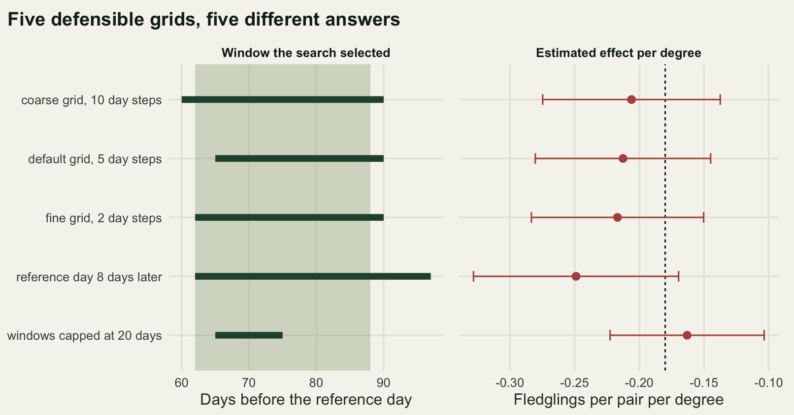
On one dataset the five grids return five windows and five effect sizes. The three grids that differ only in step size agree closely, opening at 90 days before the reference day and closing between 60 and 65, with effects of -0.2061, -0.2126 and -0.2168. Moving the reference day 8 days later, which is the same as scoring the response a week and a bit further into the season, returns a longer window and an effect of -0.2489. Capping windows at 20 days forces the search inside the true window and returns -0.1631. The largest estimate is 1.5264 times the smallest, and they span 0.0858 fledglings per pair per degree.
Set that against what the model says about its own uncertainty. The default analysis reports a 95 per cent interval 0.1356 wide, so the spread caused purely by the grid is 0.6332 of the width of the interval the analysis prints. Across 60 replicate datasets the median ratio between the largest and smallest estimate is 1.4946, and the grid spread is a median 0.5555 of the interval width, exceeding half of it in 0.55 of replicates.
The step size is the cheap part of that. Halving or doubling it moves the answer very little, because a window mean is a smooth function of its endpoints and neighbouring windows are almost the same variable. The two choices that move the answer are the ones nobody writes down: where you put the reference day, and how long a window you allow. Both encode a biological hypothesis. A reference day is a claim about when the organism integrates the weather, and a maximum window length is a claim about how long that integration can run. Neither is a tuning parameter, and neither should be chosen because it improved the fit.
What none of these checks can see
All four checks ask one question in four ways: is this window a statistical artefact? None of them asks whether the window means anything biologically, and the difference is not a philosophical one. It is measurable, so measure it.
Give the response a driver that is a nonlinear function of temperature. Nestlings die when it gets hot, so the true driver is the number of days in the true window on which the temperature exceeds 22 degrees, and each such day costs 0.12 fledglings per pair. Nothing else changes: the same weather, the same window, the same search. Then fit two models on the same 35 search years, one searching windows of mean temperature and one searching windows of hot day counts with the critical temperature itself on a grid, and score both on 15 held-out years.
crit_true <- 22
c_hot <- -0.12
sd_hot <- 0.12
n_yr5 <- 50; n_search5 <- 35
crit_grid <- seq(18, 26, by = 1)
warming <- 2
n_rep5 <- 40

count_cs <- function(temp, crit) cumzero((temp > crit) * 1)
count_from <- function(cs, g, ref = ref_day) {
  i1 <- ref - g$open; i2 <- ref - g$close
  cs[, i2 + 1, drop = FALSE] - cs[, i1, drop = FALSE]
}

set.seed(500)
big <- sim_climate(600)
big_now <- lapply(crit_grid, function(cv) count_cs(big$temp, cv))
big_warm <- lapply(crit_grid, function(cv) count_cs(big$temp + warming, cv))
true_change <- c_hot * (mean(rowSums(big$temp[, true_cols] + warming > crit_true)) -
                          mean(rowSums(big$temp[, true_cols] > crit_true)))

fit_pair <- function(cl) {
  hot <- rowSums(cl$temp[, true_cols] > crit_true)
  y <- 4 + c_hot * hot + rnorm(n_yr5, 0, sd_hot)
  tr <- seq_len(n_search5); te <- setdiff(seq_len(n_yr5), tr)
  Wm <- win_means(cumzero(cl$temp), grid5)
  sm <- search_windows(Wm[tr, ], y[tr])
  xm <- Wm[, sm$j]
  pm <- mean(y[tr]) - sm$slope * mean(xm[tr]) + sm$slope * xm
  r2o_m <- 1 - sum((y[te] - pm[te])^2) / sum((y[te] - mean(y[te]))^2)
  bj <- 0; bcv <- 0; br2 <- -1; bsl <- 0; bx <- NULL
  for (k in seq_along(crit_grid)) {
    Cm <- count_from(count_cs(cl$temp, crit_grid[k]), grid5)
    st <- search_windows(Cm[tr, ], y[tr])
    if (st$r2 > br2) {
      br2 <- st$r2; bcv <- k; bj <- st$j; bsl <- st$slope; bx <- Cm[, st$j]
    }
  }
  pt <- mean(y[tr]) - bsl * mean(bx[tr]) + bsl * bx
  r2o_t <- 1 - sum((y[te] - pt[te])^2) / sum((y[te] - mean(y[te]))^2)
  dnow <- mean(count_from(big_now[[bcv]], grid5[bj, , drop = FALSE]))
  dwarm <- mean(count_from(big_warm[[bcv]], grid5[bj, , drop = FALSE]))
  list(y = y, sm = sm, r2o_m = r2o_m, r2o_t = r2o_t,
       mean_open = grid5$open[sm$j], mean_close = grid5$close[sm$j],
       thr_open = grid5$open[bj], thr_close = grid5$close[bj],
       crit = crit_grid[bcv], thr_r2 = br2,
       pred_mean = sm$slope * warming, pred_thr = bsl * (dwarm - dnow),
       Wm = Wm, tr = tr)
}

set.seed(501)
f5 <- fit_pair(sim_climate(n_yr5))
p_rand5 <- (1 + sum(perm_max_r2(f5$Wm[f5$tr, ], f5$y[f5$tr], n_perm) >= f5$sm$r2)) /
  (n_perm + 1)
round(c(years = n_yr5, search_years = n_search5, replicates = n_rep5,
        critical_temp = crit_true, effect_per_hot_day = c_hot,
        response_noise_sd = sd_hot,
        mean_window_open = f5$mean_open, mean_window_close = f5$mean_close,
        mean_window_r2 = f5$sm$r2,
        mean_window_randomisation_p = p_rand5,
        mean_window_held_out_r2 = f5$r2o_m), 4)
years search_years
50.0000 35.0000
replicates critical_temp
40.0000 22.0000
effect_per_hot_day response_noise_sd
-0.1200 0.1200
mean_window_open mean_window_close
85.0000 60.0000
mean_window_r2 mean_window_randomisation_p
0.4851 0.0050
mean_window_held_out_r2
0.2035 round(c(threshold_window_open = f5$thr_open, threshold_window_close = f5$thr_close,
estimated_critical_temp = f5$crit, threshold_r2 = f5$thr_r2,
threshold_held_out_r2 = f5$r2o_t), 4) threshold_window_open threshold_window_close estimated_critical_temp
95.0000 60.0000 22.0000
threshold_r2 threshold_held_out_r2
0.7689 0.6534 On this run the mean temperature search passes every check in this post. It selects a window opening 85 days before the reference day and closing at 60, close to the truth. It reports an R-squared of 0.4851, survives the randomisation test with a p-value of 0.005, and scores 0.2035 on years it has never seen, above the noise threshold check 3 established. Nothing here is a false positive: the window is real, it is in the right place, and the response really does fall in warm springs. The model is also wrong about why, and that turns out to matter as soon as it is asked a question about a climate it has not seen.
set.seed(502)
c5 <- do.call(rbind, lapply(seq_len(n_rep5), function(i) {
  z <- fit_pair(sim_climate(n_yr5))
  data.frame(r2 = z$sm$r2, p = z$sm$p, r2o_m = z$r2o_m, r2o_t = z$r2o_t,
             crit = z$crit, pm = z$pred_mean, pt = z$pred_thr)
}))
round(c(warming_degrees = warming,
        hot_days_now = mean(rowSums(big$temp[, true_cols] > crit_true)),
        hot_days_warmed = mean(rowSums(big$temp[, true_cols] + warming > crit_true)),
        true_change = true_change,
        median_mean_model_change = median(c5$pm),
        median_threshold_model_change = median(c5$pt),
        mean_model_pct_of_truth = 100 * median(c5$pm) / true_change,
        threshold_model_pct_of_truth = 100 * median(c5$pt) / true_change,
        mean_model_error_pct = 100 * (median(c5$pm) / true_change - 1),
        threshold_model_error_pct = 100 * (median(c5$pt) / true_change - 1)), 4)
warming_degrees hot_days_now
2.0000 1.9183
hot_days_warmed true_change
6.9150 -0.5996
median_mean_model_change median_threshold_model_change
-0.3483 -0.6045
mean_model_pct_of_truth threshold_model_pct_of_truth
58.0904 100.8108
mean_model_error_pct threshold_model_error_pct
-41.9096 0.8108 round(c(median_mean_window_r2 = median(c5$r2),
naive_p_below_05 = mean(c5$p < 0.05),
median_mean_held_out_r2 = median(c5$r2o_m),
median_threshold_held_out_r2 = median(c5$r2o_t),
critical_temp_recovered = mean(c5$crit == crit_true)), 4) median_mean_window_r2 naive_p_below_05
0.5043 1.0000
median_mean_held_out_r2 median_threshold_held_out_r2
0.2135 0.6768
critical_temp_recovered
1.0000 Warm every day by 2 degrees, which is a mid-century projection rather than a fantasy, and ask both models what happens to breeding output. The number of days above 22 degrees in the true window rises from 1.9183 to 6.915, because the threshold sits in the tail of the daily distribution and warming drags the whole distribution through it. The true loss is 0.5996 fledglings per pair. The mean temperature model, which knows only that output falls by a fixed amount per degree of window mean, predicts a loss of 0.3483: that is 58.0904 per cent of the truth, an error of 41.9096 per cent in the direction that matters. The threshold model, fitted on exactly the same 35 years, predicts 0.6045, which is 100.8108 per cent of the truth.
Across 40 replicates the pattern holds. The mean temperature window has a median R-squared of 0.5043 and is significant at the 5 per cent level in every replicate, so no check based on significance would ever have flagged it. Its median held-out R-squared is 0.2135; the threshold model’s is 0.6768, so the out-of-sample comparison does distinguish them, but only because someone wrote the threshold model down. The search over critical temperatures recovers the true 22 degrees in all 40 replicates of this run, which says the data contain the mechanism and were simply never asked.
That is the boundary of all four checks, stated as plainly as it can be. They test whether a window is an artefact of searching. They cannot test whether the summary statistic inside the window is the one the organism responds to, because a mean and a count of exceedances move together across the years you observed, and diverge only outside them. Every extrapolation to a warmer climate is a claim about that divergence. A linear window model that passes all four checks will still under-predict the loss by more than a third if the real mechanism is a threshold, and the sign of the error is not random: a convex mechanism read through a linear model always under-predicts what warming does.
There is a second thing the checks cannot see, and it needs no simulation. Every window in this post was scored against a response measured on the same calendar. Real populations shift their timing, so the weather in a fixed window before a fixed reference day is not the weather the organism experienced when the birds bred three weeks earlier than usual. That is a mis-specified predictor, not a mis-specified test, and no amount of held-out data will report it.
Where to go next
Two of these four checks are really the same check applied at different levels: something was selected from a large set, and the reported fit does not know it. The window search is one instance, and comparing a table of candidate models is another. Checking a multi-model analysis runs the equivalent exercise on a model set: how much of a weight is selection, what happens to an averaged coefficient when the truth is not in the set, and what a held-out score does to the whole procedure.
If you have daily weather and a mechanism in mind, the better move is often to skip the search entirely. The degree day post builds a predictor from a stated biological model and estimates one or two parameters, which is a much smaller search and a much easier thing to defend.
References
van de Pol M, Bailey LD, McLean N, Rijsdijk L, Lawson CR, Brouwer L 2016 Methods in Ecology and Evolution 7(10):1246-1257 (10.1111/2041-210X.12590)
Bailey LD, van de Pol M 2016 PLoS ONE 11(12):e0167980 (10.1371/journal.pone.0167980)
Stenseth NC, Ottersen G, Hurrell JW, Mysterud A, Lima M, Chan KS, Yoccoz NG, Adlandsvik B 2003 Proceedings of the Royal Society B 270(1529):2087-2096 (10.1098/rspb.2003.2415)
Burnham KP, Anderson DR 2002 Model Selection and Multimodel Inference: A Practical Information-Theoretic Approach. Springer, ISBN 978-0-387-95364-9