library(ggplot2)

te_paper  <- "#f5f4ee"
te_ink    <- "#16241d"
te_body   <- "#2c3a31"
te_forest <- "#275139"
te_rust   <- "#b5534e"
te_gold   <- "#c9b458"
te_line   <- "#dad9ca"

theme_datasheet <- function() {
  theme_minimal(base_size = 12) +
    theme(plot.background  = element_rect(fill = te_paper, colour = NA),
          panel.background = element_rect(fill = te_paper, colour = NA),
          panel.grid.major = element_line(colour = te_line, linewidth = 0.3),
          panel.grid.minor = element_blank(),
          text             = element_text(colour = te_body),
          plot.title       = element_text(colour = te_ink, face = "bold"),
          plot.subtitle    = element_text(colour = te_body),
          axis.text        = element_text(colour = te_body))
}Tree ring detrending and the segment length curse
R
dendrochronology
time series
palaeoecology
detrending
ecology tutorial
Detrending tree ring series removes climate at periods longer than each series. Measuring the segment length curse, EPS and regional curves for ecologists in R.
A forest ecologist has cores from a few hundred pines on a dry ridge. The living trees are about eighty years old, and a scatter of stumps and beams pushes the record back a thousand years. Every core is measured, cross-dated, and then detrended: a curve is fitted to each series to remove the age trend, the tendency of a tree to lay down wide rings when it is young and narrow ones when it is old. The indices are averaged by calendar year into a chronology. The chronology tracks wet and dry years beautifully and shows no long-term change at all, and the discussion section says that growth on the ridge has been stable for a millennium.
That last sentence is not a finding. A curve fitted to an eighty year series cannot tell an age trend from a slow climate change that happens to fall inside the same eighty years, and it removes both. Averaging many such series does not bring the slow change back, because every series has had it taken out in the same way. Cook, Briffa, Meko, Graybill and Funkhouser called this the segment length curse in 1995: the longest period of climate variation a standard chronology can hold is set by the length of the individual series, not by the length of the chronology.
This post measures the curse directly. A detrending curve is a linear operator, so the fraction of climate variance it lets through at each period can be computed exactly rather than guessed, and the calculation can be checked against a forest of simulated trees. The same forest then answers two practical questions: whether the expressed population signal, the usual quality statistic for a chronology, notices what has been removed, and when regional curve standardisation, the usual cure, is worse than the disease.
The result runs the other way from detrending and bandwidth in early warning signals. There, four defensible detrending choices were applied to one collapsing series and the autocorrelation warning survived all four; the analyst’s choice moved the number but not the verdict. Here the choice decides the verdict, and no bandwidth rescues it, because the limit is a property of the series length. Checking a climate window analysis met a milder form of the same trade when it detrended a warming temperature record and lost the part of the driver that arrived through the trend. The frequency language used below is the language of spectral analysis of population cycles, and the detrending spline is a close relative of the penalised spline in penalised regression splines from scratch: the same trade between fit and a roughness penalty, with a knot at every ring and the penalty on the second derivative itself.
A detrending curve is a filter with a computable response
Everything below works on the logarithm of ring width, so that an age trend and a climate effect add, and an index is the difference between the log width and the fitted curve. This is the log form of the ratio index most chronologies use. Two detrending curves are compared. The first is a straight line in log width, which is an exponential decline in raw width and the stiffest curve that still removes an age trend. The second is the flexible default described in Cook and Kairiukstis (1990): a cubic smoothing spline whose response falls to one half at a period of 67 per cent of the series length.
Both curves are linear in the data. For a series of a given length there is a fixed matrix that turns the measured widths into indices, and that matrix is all that is needed. If every tree in a chronology has the same length and the start years are spread evenly, the chronology is a moving average of those index rows, and its response to a sine wave of any period follows from one double sum over the matrix. Squared, that response is the fraction of climate variance at that period that survives into the chronology.
spline_resid <- function(seg_len, frac = 0.67) {
  cut_period <- frac * seg_len
  lam <- (cut_period / (2 * pi))^4 / (seg_len - 1)^3
  age <- seq_len(seg_len)
  smooth_mat <- sapply(age, function(j) {
    unit <- numeric(seg_len); unit[j] <- 1
    fitted(smooth.spline(age, unit, lambda = lam, all.knots = TRUE))
  })
  diag(seg_len) - smooth_mat
}
line_resid <- function(seg_len) {
  x_mat <- cbind(1, seq_len(seg_len))
  diag(seg_len) - x_mat %*% solve(crossprod(x_mat), t(x_mat))
}
chron_gain <- function(r_mat, period) {
  seg_len <- nrow(r_mat)
  lag_mat <- outer(seq_len(seg_len), seq_len(seg_len), function(a, b) b - a)
  vapply(period, function(p) sum(r_mat * cos(2 * pi * lag_mat / p)) / seg_len, 0)
}

seg_short <- 80
seg_long  <- 250
r_list <- list(line_80 = line_resid(seg_short), spline_80 = spline_resid(seg_short),
               line_250 = line_resid(seg_long), spline_250 = spline_resid(seg_long))

n_check   <- 600
p_check   <- 0.67 * seg_short
y_check   <- sin(2 * pi * seq_len(n_check) / p_check)
fit_check <- smooth.spline(seq_len(n_check), y_check,
                           lambda = (p_check / (2 * pi))^4 / (n_check - 1)^3,
                           all.knots = TRUE)
mid_check  <- 150:450
gain_check <- unname(coef(lm(fitted(fit_check)[mid_check] ~ y_check[mid_check]))[2])

period_grid <- exp(seq(log(10), log(1000), length.out = 120))
gain_tab <- do.call(rbind, lapply(names(r_list), function(nm)
  data.frame(method = nm, period = period_grid,
             retained = chron_gain(r_list[[nm]], period_grid)^2)))

p_focus  <- 200
ret_200  <- vapply(r_list, function(r_mat) chron_gain(r_mat, p_focus)^2, 0)
half_period <- exp(vapply(r_list, function(r_mat)
  uniroot(function(lp) chron_gain(r_mat, exp(lp))^2 - 0.5,
          c(log(12), log(900)))$root, 0))
half_frac <- half_period / c(seg_short, seg_short, seg_long, seg_long)
The spline’s stiffness is set through its penalty, and smooth.spline() rescales the ages to the unit interval before applying it, which is why the penalty above is divided by the cube of the series length. That conversion is easy to get wrong, so it was checked on a long sine wave with a period of 67 per cent of eighty years: the fitted spline reproduces the wave with an amplitude gain of 0.5000, which is the one half the definition asks for.
span_bf <- 1200
sig_bf  <- sin(2 * pi * seq_len(span_bf + seg_short) / p_focus)
acc_bf  <- numeric(span_bf + seg_short)
cnt_bf  <- numeric(span_bf + seg_short)
for (st in seq_len(span_bf)) {
  yr_bf <- st:(st + seg_short - 1)
  acc_bf[yr_bf] <- acc_bf[yr_bf] + r_list$line_80 %*% sig_bf[yr_bf]
  cnt_bf[yr_bf] <- cnt_bf[yr_bf] + 1
}
chron_bf <- acc_bf / cnt_bf
mid_bf   <- 300:900
ret_bf   <- unname(coef(lm(chron_bf[mid_bf] ~ sig_bf[mid_bf]))[2])^2
The double sum is also an assertion until it is tested, so a brute force chronology was built from 1200 staggered eighty year trees, each carrying nothing but a sine wave with a period of 200 years and each detrended with its own straight line. The variance retained in the middle of that chronology is 0.002136, and the double sum gives 0.002136.
At a period of 200 years, a chronology of eighty year trees keeps 0.0021 of the climate variance under the straight line and 0.000012 under the 67 per cent spline. With 250 year trees the straight line keeps 0.835 and the spline 0.047. A two century swing in climate is, for practical purposes, absent from any chronology built from eighty year series, and whether it survives in 250 year series depends on which curve is used.
The cleanest summary is the period at which half the variance is retained. For the straight line it is 79.3 years with eighty year trees and 247.7 years with 250 year trees, that is 0.991 and 0.991 of the series length, the same fraction at both lengths to three decimals. For the 67 per cent spline it is 35.4 and 110.6 years, 0.442 and 0.442 of the length. Even the straight line cannot hold variance at periods much beyond the length of one tree, and the flexible default gives up at less than half of it.
gain_tab$curve <- ifelse(startsWith(gain_tab$method, "line"), "straight line in log width",
                         "spline, 50 per cent at 0.67 of length")
gain_tab$length <- ifelse(endsWith(gain_tab$method, "_80"), "80 year series", "250 year series")
gain_tab$length <- factor(gain_tab$length, levels = c("80 year series", "250 year series"))

ggplot(gain_tab, aes(period, retained, colour = length, linetype = curve)) +
  geom_vline(xintercept = p_focus, colour = te_line, linewidth = 0.8) +
  geom_hline(yintercept = 0.5, linetype = "dotted", colour = te_body, linewidth = 0.4) +
  geom_line(linewidth = 0.9) +
  scale_x_log10(breaks = c(10, 20, 50, 100, 200, 500, 1000)) +
  scale_colour_manual(values = c(te_rust, te_forest), name = NULL) +
  scale_linetype_manual(values = c("dashed", "solid"), name = NULL) +
  labs(x = "period of the climate variation (years, log scale)",
       y = "fraction of variance retained",
       title = "Detrending is a high pass filter",
       subtitle = "grey line: a period of two hundred years; dotted: half the variance") +
  theme_datasheet() +
  theme(legend.position = "bottom", legend.box = "vertical",
        legend.key.width = unit(2, "lines"))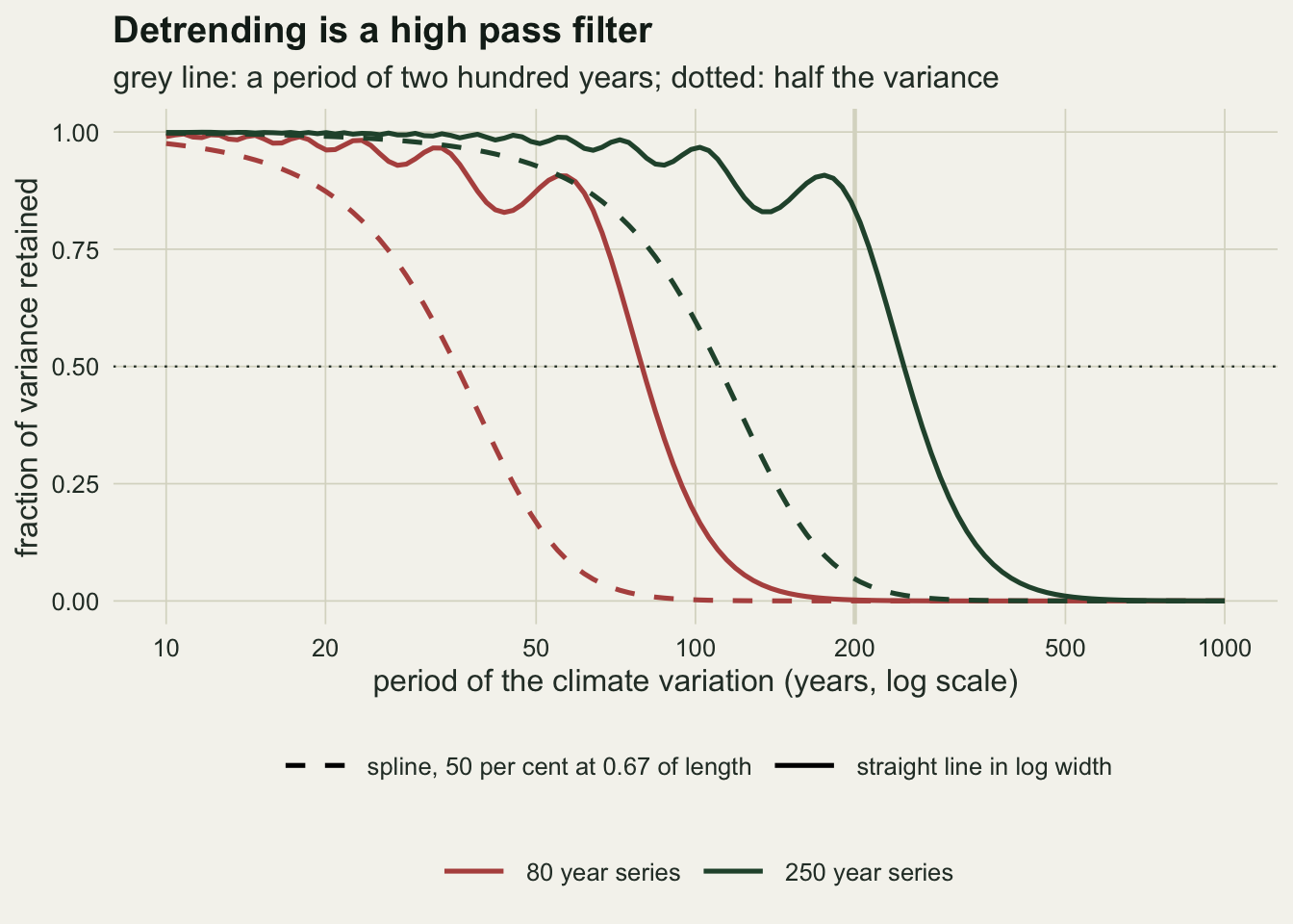
A flat millennium is an output of the procedure
The transfer function is exact but abstract. A simulated forest makes it concrete and adds the things a real chronology has: trees with different growth levels and different age trends, climate that varies from year to year as well as over centuries, and noise that belongs to each tree alone.
All the constants below were fixed before the simulation ran. The true climate over a thousand calendar years is a linear rise of 0.4 log units across the millennium, a 400 year swing with an amplitude of 0.3, a 170 year swing with an amplitude of 0.2, and year to year variation from a first order autoregressive process with a correlation of 0.3 and a standard deviation of 0.25. Each tree has its own growth level, standard deviation 0.2, and its own exponential age decline, mean 0.006 log units per year with a standard deviation of 0.0015, plus independent noise with a standard deviation of 0.35. Start years are spread evenly with a little jitter so that about 15 trees cover every calendar year, whatever the series length. The long-term part of a chronology is read with a spline whose response is one half at 100 years and compared with the noise-free long-term history itself, which contains nothing shorter than 170 years.
n_cal      <- 1000
cal_yr     <- seq_len(n_cal)
ramp_total <- 0.4
low_true   <- function(yr) ramp_total * (yr - n_cal / 2) / n_cal +
  0.3 * sin(2 * pi * yr / 400) + 0.2 * sin(2 * pi * yr / 170 + 1)
rep_target <- 15
tree_sd    <- 0.35
ar_phi     <- 0.3
inter_sd   <- 0.25
level_sd   <- 0.2
slope_mean <- -0.006
slope_sd   <- 0.0015
lp_period  <- 100
lp_lam     <- (lp_period / (2 * pi))^4 / (n_cal - 1)^3
lowpass <- function(x) fitted(smooth.spline(cal_yr, x, lambda = lp_lam, all.knots = TRUE))

sim_forest <- function(seg_len, level_grad = 0, with_low = TRUE, noise = tree_sd) {
  yrs  <- (2 - seg_len):(n_cal + seg_len - 1)
  wig  <- as.numeric(arima.sim(list(ar = ar_phi), n = length(yrs),
                               sd = inter_sd * sqrt(1 - ar_phi^2)))
  clim <- wig + if (with_low) low_true(yrs) else 0
  n_tree  <- round(rep_target * (n_cal + seg_len - 1) / seg_len)
  spacing <- (n_cal + seg_len - 1) / n_tree
  start_yr <- floor(seq(2 - seg_len, n_cal, length.out = n_tree) +
                 runif(n_tree, -spacing / 2, spacing / 2))
  start_yr <- pmin(pmax(start_yr, 2 - seg_len), n_cal)
  level <- rnorm(n_tree, 0, level_sd) + level_grad * (start_yr - n_cal / 2) / n_cal
  slope <- rnorm(n_tree, slope_mean, slope_sd)
  age   <- seq_len(seg_len)
  clean <- t(vapply(seq_len(n_tree), function(i)
    level[i] + slope[i] * age + clim[start_yr[i] - yrs[1] + age], numeric(seg_len)))
  width <- clean + matrix(rnorm(n_tree * seg_len, 0, noise), n_tree)
  list(width = width, clean = clean, start_yr = start_yr, seg_len = seg_len,
       clim = clim[yrs >= 1 & yrs <= n_cal],
       low = if (with_low) low_true(cal_yr) else 0 * cal_yr)
}
build_chron <- function(forest, index) {
  acc <- numeric(n_cal); cnt <- numeric(n_cal)
  for (i in seq_len(nrow(index))) {
    yr <- forest$start_yr[i] + seq_len(forest$seg_len) - 1
    ok <- yr >= 1 & yr <= n_cal
    acc[yr[ok]] <- acc[yr[ok]] + index[i, ok]
    cnt[yr[ok]] <- cnt[yr[ok]] + 1
  }
  acc / cnt
}
std_index <- function(forest, r_mat) forest$width %*% r_mat
rcs_index <- function(forest) sweep(forest$width, 2, colMeans(forest$width))
low_metrics <- function(chron, forest) {
  low_c <- lowpass(chron - mean(chron))
  low_t <- forest$low - mean(forest$low)
  c(r_low = cor(low_c, low_t), sd_ratio = sd(low_c) / sd(low_t),
    rmse_low = sqrt(mean((low_c - low_t)^2)),
    r_high = cor(chron - lowpass(chron), forest$clim - lowpass(forest$clim)))
}

n_forest <- 200
set.seed(4217)
forest_out <- replicate(n_forest, {
  f_80  <- sim_forest(seg_short)
  f_250 <- sim_forest(seg_long)
  c(line_80    = low_metrics(build_chron(f_80, std_index(f_80, r_list$line_80)), f_80),
    spline_80  = low_metrics(build_chron(f_80, std_index(f_80, r_list$spline_80)), f_80),
    line_250   = low_metrics(build_chron(f_250, std_index(f_250, r_list$line_250)), f_250),
    spline_250 = low_metrics(build_chron(f_250, std_index(f_250, r_list$spline_250)), f_250),
    rcs_80     = low_metrics(build_chron(f_80, rcs_index(f_80)), f_80))
})
fm  <- rowMeans(forest_out)
fse <- apply(forest_out, 1, sd) / sqrt(n_forest)
sd_low_true <- sd(low_true(cal_yr))
The true long-term history has a standard deviation of 0.268 log units. Averaged over 200 simulated forests, the chronology of eighty year trees detrended with a straight line has a long-term standard deviation of 0.061 times that, and with the 67 per cent spline 0.020 times. The correlation between the smoothed chronology and the true long-term history is 0.332 and 0.096 respectively, with Monte Carlo standard errors of 0.004 and 0.007. With 250 year trees the straight line keeps a standard deviation ratio of 0.491 and the spline 0.176.
Meanwhile the year to year signal is kept equally well by all four. The correlation between the high frequency part of the chronology and the high frequency part of the true climate is 0.935 for eighty year trees with a straight line, 0.923 with the spline, and 0.939 and 0.937 for the 250 year trees. Every chronology in the comparison is an equally good record of wet and dry years. They differ only in the part of the record that the discussion section was about.
set.seed(3140)
show_80  <- sim_forest(seg_short)
show_250 <- sim_forest(seg_long)
show_df <- rbind(
  data.frame(year = cal_yr, value = show_80$low - mean(show_80$low),
             series = "true long-term climate"),
  data.frame(year = cal_yr, series = "80 year trees, straight line",
             value = lowpass(build_chron(show_80, std_index(show_80, r_list$line_80)))),
  data.frame(year = cal_yr, series = "250 year trees, straight line",
             value = lowpass(build_chron(show_250, std_index(show_250, r_list$line_250)))),
  data.frame(year = cal_yr, series = "80 year trees, regional curve",
             value = lowpass(build_chron(show_80, rcs_index(show_80)))))
show_df$series <- factor(show_df$series, levels = unique(show_df$series))ggplot(show_df, aes(year, value, colour = series, linewidth = series)) +
geom_hline(yintercept = 0, colour = te_line, linewidth = 0.5) +
geom_line() +
scale_colour_manual(values = c(te_ink, te_rust, te_gold, te_forest), name = NULL) +
scale_linewidth_manual(values = c(1.6, 0.9, 0.9, 0.9), name = NULL) +
labs(x = "calendar year", y = "long-term growth (log units)",
title = "The chronology is flat because the trees were short",
subtitle = "chronologies smoothed with a spline at half response at 100 years") +
guides(colour = guide_legend(nrow = 2), linewidth = guide_legend(nrow = 2)) +
theme_datasheet() +
theme(legend.position = "bottom")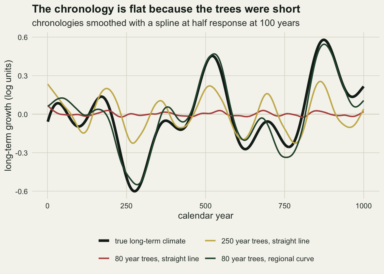
The expressed population signal does not see the loss
The standard check on a chronology is the expressed population signal of Wigley, Briffa and Jones. It takes the mean correlation between detrended series, rbar, and the number of series averaged, n, and returns n times rbar divided by one plus n minus one times rbar. It estimates the squared correlation between the chronology in hand and the chronology that an infinite number of trees would give, and a value of 0.85 is widely used as the threshold for a usable chronology.
The key phrase is the chronology that an infinite number of trees would give. That hypothetical chronology has been through the same detrending as the real one. The statistic measures how much of the tree noise has been averaged away, and it cannot measure what the detrending removed, because rbar is computed on the detrended series. The chunk below computes rbar from one forest of each series length, thins the trees to change the replication, and compares the statistic with two realised squared correlations: against the noise-free chronology built from the same trees, which is what the statistic claims to estimate, and against the true climate.
mean_rbar <- function(index, start_yr, seg_len, min_overlap = 30) {
  n_tree <- nrow(index); r_sum <- 0; n_pair <- 0
  for (i in seq_len(n_tree - 1)) for (j in (i + 1):n_tree) {
    shift <- start_yr[j] - start_yr[i]
    if (abs(shift) > seg_len - min_overlap) next
    if (shift >= 0) {
      a_seg <- index[i, (shift + 1):seg_len]; b_seg <- index[j, 1:(seg_len - shift)]
    } else {
      a_seg <- index[i, 1:(seg_len + shift)]; b_seg <- index[j, (1 - shift):seg_len]
    }
    r_sum <- r_sum + cor(a_seg, b_seg); n_pair <- n_pair + 1
  }
  r_sum / n_pair
}
eps_fun    <- function(n, rbar) n * rbar / (1 + (n - 1) * rbar)
eps_target <- 0.85
thin_frac  <- c(0.125, 0.25, 0.5, 1)

set.seed(8830)
eps_rows <- list()
for (sl in c(seg_short, seg_long)) {
  r_mat     <- if (sl == seg_short) r_list$line_80 else r_list$line_250
  forest    <- sim_forest(sl)
  idx_noisy <- std_index(forest, r_mat)
  idx_clean <- forest$clean %*% r_mat
  rbar      <- mean_rbar(idx_noisy, forest$start_yr, sl)
  for (fr in thin_frac) {
    keep <- sort(sample(nrow(idx_noisy), round(fr * nrow(idx_noisy))))
    sub_forest  <- list(start_yr = forest$start_yr[keep], seg_len = sl)
    ch_n <- build_chron(sub_forest, idx_noisy[keep, , drop = FALSE])
    ch_c <- build_chron(sub_forest, idx_clean[keep, , drop = FALSE])
    ok   <- is.finite(ch_n)
    n_rep <- mean(vapply(cal_yr, function(y)
      sum(sub_forest$start_yr <= y & sub_forest$start_yr + sl - 1 >= y), 0))
    eps_rows[[length(eps_rows) + 1]] <- data.frame(
      seg_len = sl, frac = fr, n_rep = n_rep, rbar = rbar,
      eps = eps_fun(n_rep, rbar),
      r2_pop = cor(ch_n[ok], ch_c[ok])^2,
      r2_clim = cor(ch_n[ok], forest$clim[ok])^2,
      r_low = if (all(ok)) cor(lowpass(ch_n), forest$low) else NA_real_)
  }
}
eps_tab  <- do.call(rbind, eps_rows)
full_80  <- eps_tab[eps_tab$seg_len == seg_short & eps_tab$frac == 1, ]
full_250 <- eps_tab[eps_tab$seg_len == seg_long & eps_tab$frac == 1, ]
n_need   <- function(rbar) eps_target * (1 - rbar) / (rbar * (1 - eps_target))
For the eighty year forest rbar is 0.316, so the statistic crosses 0.85 at 12.3 trees. With all trees kept the mean replication is 14.9 and the statistic is 0.873. It is accurate about what it claims to measure: the realised squared correlation between the chronology and its own noise-free version is 0.878. Against the true annual climate the squared correlation is 0.394, and the smoothed chronology correlates with the true long-term history at 0.241.
The 250 year forest has rbar 0.385, a statistic of 0.903 at a replication of 14.8, a squared correlation of 0.914 with its own noise-free version and of 0.653 with the true annual climate, and its smoothed chronology correlates with the long-term history at 0.668. Both chronologies pass the threshold. One of them has discarded almost all of the long-term climate and the other has kept a substantial part of it, and the statistic differs between them by only 0.030.
n_curve <- seq(1, 20, by = 0.25)
curve_df <- rbind(
  data.frame(n = n_curve, value = eps_fun(n_curve, full_80$rbar), forest = "80 year trees"),
  data.frame(n = n_curve, value = eps_fun(n_curve, full_250$rbar), forest = "250 year trees"))
pt_df <- rbind(
  data.frame(n = eps_tab$n_rep, value = eps_tab$r2_pop, what = "against noise-free chronology",
             forest = paste(eps_tab$seg_len, "year trees")),
  data.frame(n = eps_tab$n_rep, value = eps_tab$r2_clim, what = "against true climate",
             forest = paste(eps_tab$seg_len, "year trees")))
curve_df$forest <- factor(curve_df$forest, levels = c("80 year trees", "250 year trees"))
pt_df$forest    <- factor(pt_df$forest, levels = c("80 year trees", "250 year trees"))

ggplot(curve_df, aes(n, value)) +
  geom_hline(yintercept = eps_target, linetype = "dashed", colour = te_body, linewidth = 0.5) +
  geom_line(colour = te_forest, linewidth = 0.9) +
  geom_point(data = pt_df, aes(shape = what, colour = what), size = 2.6) +
  facet_wrap(~ forest) +
  scale_colour_manual(values = c(te_forest, te_rust), name = NULL) +
  scale_shape_manual(values = c(16, 17), name = NULL) +
  scale_y_continuous(limits = c(0, 1)) +
  labs(x = "mean number of trees per year", y = "squared correlation",
       title = "The quality statistic measures noise, not filtering",
       subtitle = "line: expressed population signal from rbar; dashed: 0.85") +
  theme_datasheet() +
  theme(legend.position = "bottom",
        strip.text = element_text(colour = te_ink, face = "bold"))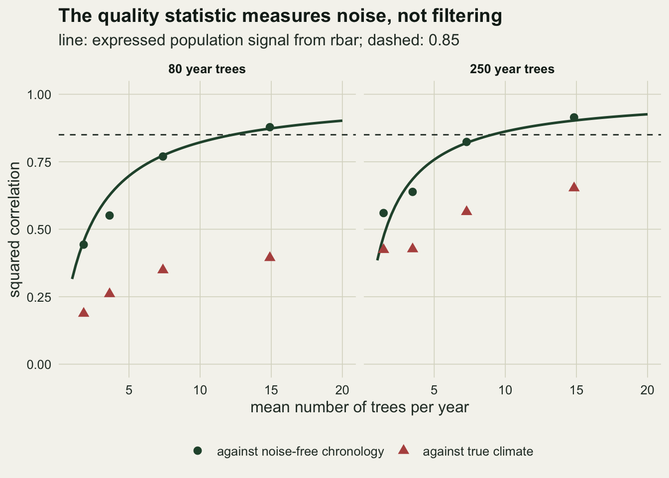
Regional curves keep the century, if the trees agree
Regional curve standardisation, set out for long chronologies by Briffa and colleagues in 1992, avoids fitting a curve to each tree. The series are aligned by cambial age, averaged into a single regional age curve, and each tree’s indices are its departures from that one curve. Because the curve does not bend to fit any individual tree, a tree that grew in a warm century keeps its wide rings. In the simulated forests above the method does what it promises: averaged over the same forests, the smoothed regional curve chronology correlates with the true long-term history at 0.971 with a standard deviation ratio of 1.002 (the smoother slightly damps the 170 year swing and lets some noise through, so a ratio near one is not exact recovery), from the same eighty year trees that the straight line reduced to 0.061.
The promise rests on an assumption: every tree follows the same age curve apart from climate and noise that averages away. In the forest above the tree levels were independent of when the trees grew. Real collections break that. Living trees on the ridge today may have grown up in an open stand after grazing ended and grown fast, while the subfossil wood came from trees that grew slowly in a closed forest; or the old wood that survived to be sampled may be a biased subset. The chunk below makes growth level drift with germination year, from zero to two log units across the millennium on a grid fixed before running, and measures the root mean square error of the smoothed chronology against the true long-term history. A second run removes all long-term climate and sets the drift at 0.5, to show what the method reports when there is nothing to find.
grad_grid <- c(0, 0.25, 0.5, 0.75, 1, 1.5, 2)
n_sweep   <- 100
set.seed(5102)
sweep_tab <- as.data.frame(t(vapply(grad_grid, function(g) {
  m_out <- replicate(n_sweep, {
    f_80 <- sim_forest(seg_short, level_grad = g)
    c(low_metrics(build_chron(f_80, rcs_index(f_80)), f_80)[["rmse_low"]],
      low_metrics(build_chron(f_80, std_index(f_80, r_list$line_80)), f_80)[["rmse_low"]])
  })
  c(grad = g, rcs = mean(m_out[1, ]), rcs_se = sd(m_out[1, ]) / sqrt(n_sweep),
    std = mean(m_out[2, ]), std_se = sd(m_out[2, ]) / sqrt(n_sweep))
}, numeric(5))))
cross_grad <- approx(sweep_tab$rcs - sweep_tab$std, sweep_tab$grad, xout = 0)$y
se_max     <- max(sweep_tab$rcs_se)

flat_grad <- 0.5
set.seed(6021)
flat_out <- replicate(n_sweep, {
  f_flat <- sim_forest(seg_short, level_grad = flat_grad, with_low = FALSE)
  ch_r <- build_chron(f_flat, rcs_index(f_flat))
  ch_s <- build_chron(f_flat, std_index(f_flat, r_list$line_80))
  c(rcs = sd(lowpass(ch_r)), std = sd(lowpass(ch_s)),
    rcs_rise = unname(coef(lm(ch_r ~ cal_yr))[2]) * n_cal)
})
flat_mean <- rowMeans(flat_out)
With no drift the regional curve chronology has a long-term error of 0.069 log units against 0.263 for straight line detrending, whose error is the long-term climate it threw away. The regional curve error grows steadily with the drift and reaches 0.583 at a drift of two log units; the largest Monte Carlo standard error in the sweep is 0.0019. The two errors are equal at a drift of about 0.88 log units per millennium, a factor of 2.4 in growth level between trees that germinated at the start and at the end of the millennium. Below that the regional curve is the better long-term record in this forest; above it the regional curve is worse than doing the thing it was invented to replace.
That comparison flatters the regional curve in one respect. Its error is not noise but a trend, and a trend is what the study reports. With the long-term climate switched off and a drift of 0.5, the straight line chronology has a long-term standard deviation of 0.0129 log units, which is the correct answer of nothing. The regional curve chronology has 0.1588 and a fitted rise of 0.504 log units across the millennium, which is the drift in the sampling returned as climate.
sweep_long <- rbind(
  data.frame(grad = sweep_tab$grad, err = sweep_tab$rcs, se = sweep_tab$rcs_se,
             method = "regional curve"),
  data.frame(grad = sweep_tab$grad, err = sweep_tab$std, se = sweep_tab$std_se,
             method = "straight line per tree"))
ggplot(sweep_long, aes(grad, err, colour = method)) +
  geom_vline(xintercept = cross_grad, linetype = "dashed", colour = te_body, linewidth = 0.5) +
  geom_line(linewidth = 0.9) +
  geom_errorbar(aes(ymin = err - 1.96 * se, ymax = err + 1.96 * se), width = 0.04) +
  geom_point(size = 2.2) +
  scale_colour_manual(values = c(te_rust, te_forest), name = NULL) +
  labs(x = "drift in growth level across the millennium (log units)",
       y = "long-term error (log units)",
       title = "Regional curves fail when the trees differ by era",
       subtitle = "eighty year trees; dashed: where the two errors meet") +
  theme_datasheet() +
  theme(legend.position = "bottom")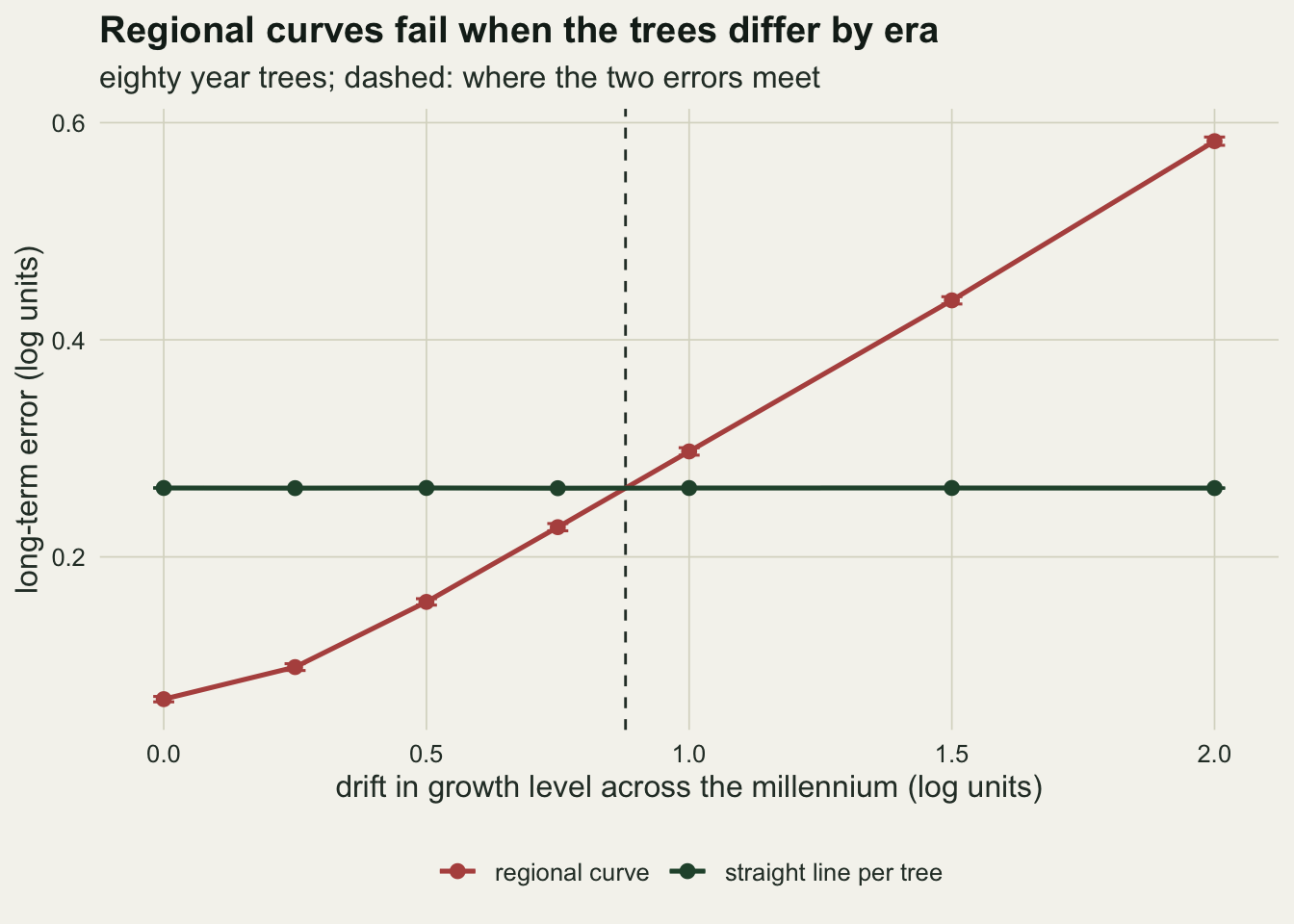
What to report
State the series lengths, not only the chronology length. A chronology spanning a thousand years made of eighty year series is, in the frequency band the discussion usually cares about, an eighty year instrument. The distribution of series lengths, and the detrending curve, together determine the longest period the chronology can carry, and the transfer function above takes a few lines of R for any curve that is linear in the data.
Report the half variance period of the detrending actually used, or show the transfer function. For a straight line fitted to each series it was 0.99 of the series length and for the 67 per cent spline 0.44 of it, so the flexible default spline keeps less than half the variance at any period longer than half a tree’s life. A statement that there is no long-term trend in a chronology built this way should be written as a statement about the method.
Do not use the expressed population signal as evidence about low frequency. It passed 0.85 for both forests while one of them had lost almost all of its long-term climate. Report it for what it is, a measure of replication against tree noise, and report the replication through time alongside it.
If regional curve standardisation is used, say how the age curve was checked for being common. Split the trees by era or by site and compare their regional curves; if living and subfossil trees grow at different levels at the same age, the long-term signal of the chronology contains that difference. Where standard and regional curve chronologies disagree at long periods, the honest statement is that the collection cannot separate climate from sampling history, not that one of the two is right.
Honest limits
The whole analysis is in log width with additive indices. Most chronologies divide raw widths by the fitted curve. A ratio index w/c is close to 1 + log(w/c) only while indices stay near one, so the two forms agree for small departures; ratio indices misbehave mainly when a fitted curve runs close to zero (a declining straight line in raw width, for instance), where small widths divided by a tiny curve inflate the variance of old rings. The straight line in log width stands in for the negative exponential and has no asymptote. A negative exponential with an asymptote has one more parameter than the straight line and was not tested; it may retain less at long periods.
Every tree in each forest has the same length, and start years are spread evenly. Real collections mix short and long series and cluster in time: the living trees crowd into the last century and the subfossil wood arrives in patches. With mixed lengths the transfer function becomes a weighted average of the individual ones and changes through the chronology, so a single half variance period describes no real collection exactly.
The signal-free and age-band methods, and the many refinements of regional curve standardisation, were not tested. The drift used against the regional curve is one simple kind of disagreement between trees, a shift in level that is linear in germination year. Differences in the shape of the age curve, or a sampling bias that depends on tree size rather than on era, would produce different errors, and the break-even drift reported here belongs to this forest and its constants, not to any real species.
The long-term climate is a fixed history of one ramp and two sine waves, and the year to year climate is a weak autoregressive process. A climate with more variance at long periods relative to short ones makes the loss under standard detrending a larger share of the total, and a climate with less makes it smaller. The retained fractions at each period do not depend on that choice; the correlations and errors of the smoothed chronologies do.
References
Cook ER, Briffa KR, Meko DM, Graybill DA, Funkhouser G 1995 The Holocene 5(2):229-237 (10.1177/095968369500500211)
Wigley TML, Briffa KR, Jones PD 1984 Journal of Climate and Applied Meteorology 23(2):201-213 (10.1175/1520-0450(1984)023<0201:OTAVOC>2.0.CO;2)
Briffa KR, Jones PD, Bartholin TS, Eckstein D, Schweingruber FH, Karlen W, Zetterberg P, Eronen M 1992 Climate Dynamics 7(3):111-119 (10.1007/BF00211153)
Cook ER, Kairiukstis LA (eds) 1990 Methods of Dendrochronology: Applications in the Environmental Sciences (ISBN 978-90-481-4060-2)