library(ggplot2)

te_pal <- list(forest = "#275139", green = "#2f8f63", sage = "#93a87f",
               clay = "#b5534e", gold = "#cda23f", line = "#dad9ca",
               ink = "#16241d", paper = "#f5f4ee")

theme_te <- function() {
  theme_minimal(base_size = 12) +
    theme(panel.grid.minor = element_blank(),
          panel.grid.major = element_line(colour = "#e7e6dc"),
          plot.background = element_rect(fill = "#f5f4ee", colour = NA),
          panel.background = element_rect(fill = "#f5f4ee", colour = NA),
          plot.title = element_text(face = "bold", colour = te_pal$ink),
          axis.title = element_text(colour = "#2c3a31"))
}Drought indices for ecologists
R
climate
drought
phenology
ecology tutorial
ggplot2
Build SPI, SPEI and a climatic water balance by hand in R, and measure how much the accumulation window, baseline and evapotranspiration decide a drought year.
An ecologist who wants drought in a model has to make it up. Temperature arrives as a number, rainfall arrives as a number, but drought is not measured by any instrument: it is constructed from a weather record by a chain of decisions, and the chain is longer than most methods sections admit. How many months of weather do you accumulate. Do you subtract evaporative demand or only count the rain. Which years do you standardise against. Each answer produces a different variable called drought, and the differences are not small.
This tutorial builds three drought indices from scratch in base R and then scores them. The trick that makes scoring possible is simulation: we generate a monthly weather record, run a soil water bucket through it to get a water stress process we know exactly, and let that stress drive the growth of two simulated species. Every index is then a proxy for something we can see. The question stops being which index is theoretically preferable and becomes which construction recovers the stress that actually acted, and by how much the wrong construction loses.
If you have read climate window analysis in R you have met the window problem already, in the version where the analyst searches over windows and the search itself inflates the result. Here the window is one of four construction choices, and the comparison is against a known truth rather than against a null. The last section is the one that matters most, because it measures the limit that no amount of index engineering removes: two species living through the same weather need different indices.
A weather record with a water stress process inside it
The weather generator is deliberately plain. Monthly precipitation is gamma distributed with a shape that stays fixed and a mean that follows a sinusoid peaking in July. Monthly temperature is a seasonal sinusoid plus an anomaly that follows a first order autoregressive process, so warm months cluster the way they do in a real record. A warming trend can be added as a linear ramp on the temperature, which is how the second half of the post gets its non-stationary record.
Potential evapotranspiration comes from Thornthwaite’s 1948 temperature-only formula, coded here in full. It builds an annual heat index from the twelve monthly mean temperatures, derives an exponent from that index by a cubic polynomial, and returns monthly demand as a power function of mean temperature. This is the crudest of the standard formulas: no radiation, no humidity, no wind, and the day length correction is left out here so the arithmetic stays visible. It is also the formula that sits inside a large fraction of published drought indices, so its behaviour is worth seeing.
The known truth is a single bucket of soil water with a fixed capacity. Each month the bucket receives the rain, gives up as much water as demand asks for or as much as it holds, whichever is less, and spills anything above capacity. Water stress in that month is the shortfall of actual evapotranspiration below potential, as a proportion of potential. That stress series is the process the indices are trying to see, and no index in this post is given access to it.
Two species then integrate the stress over different times. Each carries an exponentially weighted memory of past stress, one with a time constant of two months, standing for a shallow rooted annual that responds to the current summer, and one with a time constant of 18 months, standing for a deep rooted woody plant whose current growth still carries last year’s drought. Annual performance is measured in August and is a linear function of the standardised memory plus observation noise. The noise is set so that both species have the same signal to noise ratio, which makes the two sets of correlations directly comparable.
set.seed(20260719)

n_stat <- 150; n_warm <- 120; warm_rate <- 0.25; cap <- 100
windows <- c(1, 3, 6, 12); anchor <- 8; thresh <- -1
tau_a <- 2; tau_b <- 18; sig_e <- 12; amp <- 25
p_shape <- 2.2; ar_phi <- 0.45

sim_weather <- function(nyr, warm_per_decade = 0) {
  n <- nyr * 12
  mn <- rep(1:12, nyr); yr <- rep(seq_len(nyr), each = 12)
  p_mean <- 42 + 11 * sin(2 * pi * (mn - 4) / 12)
  precip <- rgamma(n, shape = p_shape, rate = p_shape / p_mean)
  t_seas <- 9.5 + 10.5 * cos(2 * pi * (mn - 7) / 12)
  s_a <- 1.3
  anom <- numeric(n); anom[1] <- rnorm(1, 0, s_a)
  for (i in 2:n) anom[i] <- ar_phi * anom[i - 1] + sqrt(1 - ar_phi^2) * rnorm(1, 0, s_a)
  data.frame(year = yr, month = mn, precip = precip,
             temp = t_seas + anom + warm_per_decade * (yr - 1) / 10)
}

pet_thorn <- function(temp, month, heat = NULL) {
  tpos <- pmax(temp, 0)
  if (is.null(heat)) heat <- sum((tapply(tpos, month, mean) / 5)^1.514)
  aa <- 6.75e-7 * heat^3 - 7.71e-5 * heat^2 + 1.792e-2 * heat + 0.49239
  list(pet = 16 * (10 * tpos / heat)^aa, heat = heat, a = aa)
}

water_stress <- function(precip, pet, cap) {
  n <- length(precip); ww <- cap
  st <- numeric(n); wo <- numeric(n)
  for (i in seq_len(n)) {
    avail <- ww + precip[i]
    aet <- min(pet[i], avail)
    st[i] <- if (pet[i] > 0.5) 1 - aet / pet[i] else 0
    ww <- min(cap, avail - aet)
    wo[i] <- ww
  }
  list(stress = st, water = wo)
}

ewma <- function(x, tau) {
  rho <- exp(-1 / tau); acc <- 0; out <- numeric(length(x))
  for (i in seq_along(x)) { acc <- rho * acc + (1 - rho) * x[i]; out[i] <- acc }
  out
}

w <- sim_weather(n_stat)
pt <- pet_thorn(w$temp, w$month)
w$pet <- pt$pet
w$bal <- w$precip - w$pet
ws <- water_stress(w$precip, w$pet, cap)

aug <- which(w$month == anchor)
gA <- ewma(ws$stress, tau_a)[aug]
gB <- ewma(ws$stress, tau_b)[aug]
zA <- (gA - mean(gA)) / sd(gA)
zB <- (gB - mean(gB)) / sd(gB)
yA <- 100 - amp * zA + rnorm(n_stat, 0, sig_e)
yB <- 100 - amp * zB + rnorm(n_stat, 0, sig_e)

round(c(record_years = n_stat, soil_capacity_mm = cap, memory_A_months = tau_a,
        memory_B_months = tau_b, response_amplitude = amp, response_noise_sd = sig_e,
        precip_gamma_shape = p_shape, temperature_ar1 = ar_phi), 3)
record_years soil_capacity_mm memory_A_months memory_B_months
150.00 100.00 2.00 18.00
response_amplitude response_noise_sd precip_gamma_shape temperature_ar1
25.00 12.00 2.20 0.45 round(c(mean_annual_precip = sum(w$precip) / n_stat,
mean_annual_pet = sum(w$pet) / n_stat,
thornthwaite_heat_index = pt$heat, thornthwaite_exponent = pt$a,
july_pet_minus_precip = mean(w$pet[w$month == 7]) -
mean(w$precip[w$month == 7])), 3) mean_annual_precip mean_annual_pet thornthwaite_heat_index
503.353 546.007 40.115
thornthwaite_exponent july_pet_minus_precip
1.131 44.592 print(round(tapply(ws$stress, w$month, mean), 3)) 1 2 3 4 5 6 7 8 9 10 11 12
0.000 0.000 0.000 0.000 0.009 0.098 0.315 0.369 0.344 0.196 0.035 0.003 round(c(sd_stress_A = sd(gA), sd_stress_B = sd(gB), cor_A_B = cor(gA, gB),
cor_response_A_truth = cor(yA, -zA), cor_response_B_truth = cor(yB, -zB)), 3) sd_stress_A sd_stress_B cor_A_B
0.167 0.041 0.705
cor_response_A_truth cor_response_B_truth
0.895 0.900 The record covers 150 years with 503.353 mm of precipitation and 546.007 mm of potential evapotranspiration a year on average, so demand exceeds supply annually by a small margin and by a large one in summer: July demand exceeds July precipitation by 44.592 mm. The Thornthwaite heat index is 40.115 and the exponent derived from it is 1.131. Mean monthly stress is at or near zero from January to April and negligible in May, November and December (0.009, 0.035 and 0.003), rises through June, and peaks at 0.369 in August. The soil bucket holds 100 mm.
The two species differ in how much of that stress reaches them. The short memory species carries a standard deviation of 0.167 in its August stress integral; the long memory species, smoothing over a year and a half, carries only 0.041. The two integrals correlate at 0.705, so they are neither the same variable nor independent ones. Because both responses are built from a standardised memory with the same coefficients, each correlates with its own truth at 0.895 and 0.9, and any loss below that is the fault of the index rather than of the noise.
Three indices, each coded by hand
The first index is the climatic water balance itself: precipitation minus potential evapotranspiration, accumulated over a window, in millimetres. It has a physical meaning and no statistical one.
The second is the standardised precipitation index. Accumulate precipitation over the previous \(k\) months, take all the values that fall in the same calendar month, fit a gamma distribution to them by maximum likelihood, evaluate the fitted distribution function at each observation, and map the resulting probability through the standard normal quantile function. The log-likelihood is written out rather than taken from a fitting package, and optim runs twice from the moment estimates so that the second start is close to the answer:
\[\ell(\alpha, \beta) = \sum_i \left[ (\alpha - 1)\log x_i - \beta x_i + \alpha \log \beta - \log \Gamma(\alpha) \right]\]
The third applies the same standardisation to the water balance. The gamma cannot be used here, because an accumulated water balance is routinely negative, so the distribution needs a location parameter. A three parameter log-logistic does the job and is the family the published SPEI uses, with distribution function
\[F(x) = \left[ 1 + \left( \frac{\alpha}{x - \gamma} \right)^{\beta} \right]^{-1}, \qquad x > \gamma\]
fitted here by maximum likelihood on the same pattern, with a starting location just below the smallest observation. Because the probability integral transform is monotone, both standardised indices are order preserving within a calendar month: they change the label attached to a year, never which year is drier. That will matter later.
Any standardisation machinery has to be checked before it is used. On a long stationary record the standardised indices must be approximately standard normal, so their mean should be near zero, their standard deviation near one, and the proportion of values below -1.28 near 0.1003.
accumulate <- function(x, k) {
  n <- length(x); out <- rep(NA_real_, n); cs <- cumsum(x)
  out[k:n] <- cs[k:n] - c(0, cs[seq_len(n - k)])
  out
}

gam_nll <- function(par, x) {
  sh <- exp(par[1]); rt <- exp(par[2])
  -sum((sh - 1) * log(x) - rt * x + sh * log(rt) - lgamma(sh))
}
fit_gam <- function(x) {
  mu <- mean(x); vv <- var(x)
  op <- optim(c(log(mu^2 / vv), log(mu / vv)), gam_nll, x = x,
              control = list(reltol = 1e-12, maxit = 2000))
  op <- optim(op$par, gam_nll, x = x, control = list(reltol = 1e-12, maxit = 2000))
  c(shape = exp(op$par[1]), rate = exp(op$par[2]))
}
p_gam <- function(q, p) pgamma(q, shape = p["shape"], rate = p["rate"])

ll_nll <- function(par, x) {
  al <- exp(par[1]); be <- exp(par[2]); ga <- par[3]
  z <- x - ga
  if (any(z <= 1e-8)) return(1e10)
  -sum(log(be / al) + (be - 1) * log(z / al) - 2 * log1p((z / al)^be))
}
fit_ll <- function(x) {
  ga0 <- min(x) - 0.15 * (max(x) - min(x)); z <- x - ga0
  init <- c(mean(log(z)), log(pi / (sqrt(3) * sd(log(z)))), ga0)
  op <- optim(init, ll_nll, x = x, control = list(reltol = 1e-12, maxit = 4000))
  op <- optim(op$par, ll_nll, x = x, control = list(reltol = 1e-12, maxit = 4000))
  c(alpha = exp(op$par[1]), beta = exp(op$par[2]), gamma = op$par[3])
}
p_ll <- function(q, p) 1 / (1 + (p["alpha"] / (q - p["gamma"]))^p["beta"])

standardise <- function(acc, month, fitter, cdf, ref = NULL) {
  out <- rep(NA_real_, length(acc))
  for (m in 1:12) {
    idx <- which(month == m & !is.na(acc))
    rows <- if (is.null(ref)) idx else intersect(idx, ref)
    par <- fitter(acc[rows])
    pr <- cdf(acc[idx], par)
    out[idx] <- qnorm(pmin(pmax(pr, 1e-7), 1 - 1e-7))
  }
  out
}

idx_stat <- list()
for (k in windows) {
  ap <- accumulate(w$precip, k); ab <- accumulate(w$bal, k)
  idx_stat[[paste0("bal", k)]]  <- ab
  idx_stat[[paste0("spi", k)]]  <- standardise(ap, w$month, fit_gam, p_gam)
  idx_stat[[paste0("spei", k)]] <- standardise(ab, w$month, fit_ll, p_ll)
}

check_norm <- function(tag) {
  out <- sapply(windows, function(k) {
    z <- idx_stat[[paste0(tag, k)]]
    c(mean = mean(z, na.rm = TRUE), sd = sd(z, na.rm = TRUE),
      below_1_28 = mean(z < -1.28, na.rm = TRUE))
  })
  colnames(out) <- paste0("w", windows)
  round(out, 4)
}
round(c(z_cut = -1.28, expected_tail = pnorm(-1.28)), 4)
z_cut expected_tail
-1.2800 0.1003 print(check_norm("spi")) w1 w3 w6 w12
mean -0.0012 0.0000 0.0001 0.0000
sd 0.9999 1.0003 1.0003 1.0003
below_1_28 0.1006 0.1057 0.1075 0.1034print(check_norm("spei")) w1 w3 w6 w12
mean -0.0096 -0.0080 -0.0037 -0.0037
sd 0.9863 0.9835 0.9859 0.9830
below_1_28 0.1122 0.1129 0.1025 0.1012round(fit_gam(accumulate(w$precip, 12)[aug[-1]]), 4) shape rate
27.5561 0.0547 The SPI machinery passes cleanly. At a one month window the mean is -0.0012, the standard deviation 0.9999 and the proportion below -1.28 is 0.1006 against the expected 0.1003; at twelve months the three numbers are 0, 1.0003 and 0.1034. Nothing here says the index is a good measure of drought. It says the transformation is arithmetically sound, which is the only claim it makes about itself.
The SPEI machinery is slightly off, and the direction is informative. Its standard deviation runs between 0.983 and 0.9863 across the four windows rather than sitting at one, and its mean is between -0.0096 and -0.0037 rather than zero. Three parameters fitted by maximum likelihood to 150 values shrink the tails a little, because the fitted distribution is pulled towards the sample it was fitted to. The effect is small at this record length and grows as the record shortens, which is a reason to be careful with a 30 year series and a three parameter fit. The gamma fitted to the twelve month August precipitation totals has a shape of 27.5561 and a rate of 0.0547, so the accumulated annual total is close to normal, as a sum of twelve gamma draws should be.
library(grid)
show_years <- (n_stat - 44):n_stat
zoom_years <- (n_stat - 11):n_stat
sel <- w$year %in% show_years
sez <- w$year %in% zoom_years
tt <- w$year + (w$month - 1) / 12
pan_top <- paste0("Monthly weather (mm), years ", min(zoom_years), " to ", max(zoom_years))
pan <- c("Water balance, 12 months (mm)", "SPI, 12 months", "SPEI, 12 months")
pal_rec <- c("Precipitation" = te_pal$green,
             "Potential evapotranspiration" = te_pal$clay,
             "Water balance" = te_pal$sage,
             "SPI" = te_pal$gold,
             "SPEI" = te_pal$forest)

top <- rbind(
  data.frame(t = tt[sez], value = w$precip[sez], series = "Precipitation"),
  data.frame(t = tt[sez], value = w$pet[sez], series = "Potential evapotranspiration"))
top$panel <- factor(pan_top)

rec <- rbind(
  data.frame(t = tt[sel], value = idx_stat$bal12[sel], series = "Water balance", panel = pan[1]),
  data.frame(t = tt[sel], value = idx_stat$spi12[sel], series = "SPI", panel = pan[2]),
  data.frame(t = tt[sel], value = idx_stat$spei12[sel], series = "SPEI", panel = pan[3]))
rec$panel <- factor(rec$panel, levels = pan)
zline <- data.frame(yv = c(0, thresh, thresh), panel = factor(pan, levels = pan))

p_top <- ggplot(top, aes(t, value, colour = series)) +
  geom_line(linewidth = 0.6) +
  facet_wrap(~panel, ncol = 1) +
  scale_colour_manual(values = pal_rec, name = NULL) +
  scale_x_continuous(breaks = seq(min(zoom_years), max(zoom_years), by = 2),
                     expand = expansion(mult = c(0.02, 0.03))) +
  labs(x = "Year of record", y = NULL,
       title = "One weather record, three drought indices") +
  theme_te() +
  theme(legend.position = "top",
        strip.text = element_text(colour = te_pal$ink, face = "bold"),
        plot.margin = margin(5.5, 12, 2, 5.5))

p_bot <- ggplot(rec, aes(t, value, colour = series)) +
  geom_hline(data = zline, aes(yintercept = yv), colour = te_pal$line, linewidth = 0.7) +
  geom_line(linewidth = 0.6) +
  facet_wrap(~panel, ncol = 1, scales = "free_y") +
  scale_colour_manual(values = pal_rec, guide = "none") +
  scale_x_continuous(expand = expansion(mult = c(0.02, 0.03))) +
  labs(x = paste0("Year of record, years ", min(show_years), " to ", max(show_years)),
       y = NULL) +
  theme_te() +
  theme(strip.text = element_text(colour = te_pal$ink, face = "bold"),
        plot.margin = margin(2, 12, 5.5, 5.5))

grid.newpage()
grid.rect(gp = gpar(fill = te_pal$paper, col = NA))
pushViewport(viewport(layout = grid.layout(2, 1, heights = unit(c(1.35, 2), "null"))))
print(p_top, vp = viewport(layout.pos.row = 1, layout.pos.col = 1))
print(p_bot, vp = viewport(layout.pos.row = 2, layout.pos.col = 1))
popViewport()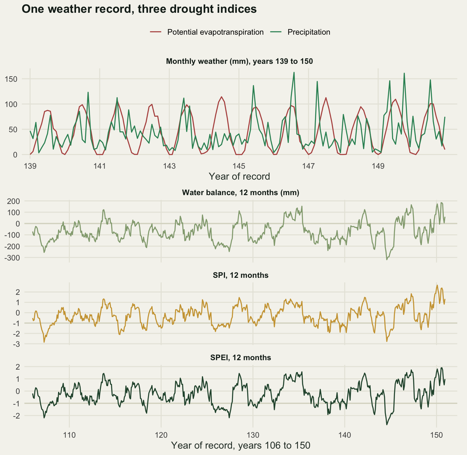
The accumulation window is a choice about the organism
An index at a one month window asks whether this month was dry. At twelve months it asks whether the year was dry. Those are different questions and they have different answers, which is easy to say and easy to underestimate. The correlation matrix across windows measures the size of the disagreement directly, and the drought year classification measures what survives it.
grab <- function(tag) {
  M <- sapply(windows, function(k) idx_stat[[paste0(tag, k)]][aug])
  colnames(M) <- paste0("w", windows)
  M
}
for (tag in c("bal", "spi", "spei")) {
  cat(tag, "\n"); print(round(cor(grab(tag), use = "pair"), 3))
}
bal
w1 w3 w6 w12
w1 1.000 0.583 0.464 0.340
w3 0.583 1.000 0.774 0.626
w6 0.464 0.774 1.000 0.815
w12 0.340 0.626 0.815 1.000
spi
w1 w3 w6 w12
w1 1.000 0.496 0.392 0.261
w3 0.496 1.000 0.752 0.610
w6 0.392 0.752 1.000 0.805
w12 0.261 0.610 0.805 1.000
spei
w1 w3 w6 w12
w1 1.000 0.512 0.422 0.315
w3 0.512 1.000 0.752 0.608
w6 0.422 0.752 1.000 0.818
w12 0.315 0.608 0.818 1.000jaccard <- function(tag) {
M <- grab(tag)
d1 <- which(M[, 1] < thresh); d12 <- which(M[, 4] < thresh)
c(n_window_1 = length(d1), n_window_12 = length(d12),
shared = length(intersect(d1, d12)),
overlap = length(intersect(d1, d12)) / length(union(d1, d12)))
}
round(c(drought_threshold = thresh), 2)drought_threshold
-1 print(round(rbind(spi = jaccard("spi"), spei = jaccard("spei")), 3)) n_window_1 n_window_12 shared overlap
spi 23 24 6 0.146
spei 26 25 7 0.159The August values of the SPEI correlate at 0.512 between the one month and three month windows, at 0.818 between six and twelve months, and at 0.315 between the extremes. The SPI matrix is much the same, with 0.261 between the extremes. Two analysts who each report the standardised precipitation index, one at a month and one at a year, are reporting variables whose August values correlate at 0.261.
Classification makes the point harder to argue with. Using a threshold of -1, the one month SPEI calls 26 of the 150 Augusts a drought and the twelve month SPEI calls 25, which sounds like agreement until you ask which ones: only 7 years appear on both lists, an overlap of 0.159. The SPI behaves the same way, with 23 and 24 years flagged, 6 shared and an overlap of 0.146. Only about a sixth of the years flagged by one window or the other are flagged by both. A paper that reports the number of drought years in a region has reported a property of its own accumulation window at least as much as a property of the climate.
Scoring the windows against the truth
Nothing above says which window is right, because nothing above involves an organism. Now bring the two simulated species back and correlate every index and window combination with their annual performance.
combos <- expand.grid(k = windows, idx = c("bal", "spi", "spei"), stringsAsFactors = FALSE)
X <- sapply(seq_len(nrow(combos)),
            function(j) idx_stat[[paste0(combos$idx[j], combos$k[j])]][aug])
score <- rbind(
  A = as.numeric(cor(yA, X, use = "pair")),
  B = as.numeric(cor(yB, X, use = "pair")))
colnames(score) <- paste0(combos$idx, combos$k)
print(round(score, 3))
bal1 bal3 bal6 bal12 spi1 spi3 spi6 spi12 spei1 spei3 spei6 spei12
A 0.530 0.777 0.780 0.682 0.477 0.806 0.780 0.684 0.492 0.789 0.786 0.684
B 0.301 0.486 0.557 0.607 0.299 0.499 0.523 0.579 0.295 0.488 0.555 0.617best <- data.frame(
species = c("A", "B"),
best_combo = colnames(score)[apply(score, 1, which.max)],
best_r = round(apply(score, 1, max), 3))
print(best) species best_combo best_r
A A spi3 0.806
B B spei12 0.617round(c(window_cost_A = score["A", "spi3"] - score["A", "spi12"],
index_gap_A = score["A", "spi3"] - score["A", "spei3"]), 3)window_cost_A index_gap_A
0.122 0.017 set.seed(909)
n_redraw <- 200
winA <- winB <- integer(nrow(combos))
for (r in seq_len(n_redraw)) {
ya <- 100 - amp * zA + rnorm(n_stat, 0, sig_e)
yb <- 100 - amp * zB + rnorm(n_stat, 0, sig_e)
ja <- which.max(cor(ya, X, use = "pair")); winA[ja] <- winA[ja] + 1L
jb <- which.max(cor(yb, X, use = "pair")); winB[jb] <- winB[jb] + 1L
}
noise_free <- rbind(A = as.numeric(cor(-zA, X, use = "pair")),
B = as.numeric(cor(-zB, X, use = "pair")))
colnames(noise_free) <- colnames(score)
tallies <- data.frame(combo = colnames(score), redraws = n_redraw,
win_A = winA / n_redraw, win_B = winB / n_redraw,
nf_A = round(noise_free["A", ], 3),
nf_B = round(noise_free["B", ], 3))
print(tallies[tallies$win_A > 0 | tallies$win_B > 0, ], row.names = FALSE) combo redraws win_A win_B nf_A nf_B
bal6 200 0.005 0 0.864 0.622
spi3 200 0.005 0 0.857 0.572
spei3 200 0.560 0 0.877 0.560
spei6 200 0.430 0 0.875 0.630
spei12 200 0.000 1 0.755 0.724print(round(noise_free, 3)) bal1 bal3 bal6 bal12 spi1 spi3 spi6 spi12 spei1 spei3 spei6 spei12
A 0.565 0.847 0.864 0.75 0.525 0.857 0.828 0.711 0.554 0.877 0.875 0.755
B 0.321 0.546 0.622 0.71 0.315 0.572 0.598 0.681 0.319 0.560 0.630 0.724library(grid)
cm <- cor(grab("spei"), use = "pair")
lab <- paste0(windows, " mo")
dimnames(cm) <- list(lab, lab)
tile <- expand.grid(a = factor(lab, levels = lab), b = factor(lab, levels = lab))
tile$r <- as.vector(cm)
p1 <- ggplot(tile, aes(a, b, fill = r)) +
geom_tile(colour = te_pal$paper, linewidth = 1) +
geom_text(aes(label = sprintf("%.2f", r)), colour = te_pal$ink, size = 3.4) +
scale_fill_gradient(low = te_pal$paper, high = te_pal$green,
limits = c(0, 1), name = "Correlation") +
labs(x = "Accumulation window", y = "Accumulation window",
title = "One index, four windows") +
theme_te() + theme(legend.position = "none")
sc <- data.frame(window = rep(combos$k, 2),
index = rep(combos$idx, 2),
species = rep(c("Short memory: 2 months", "Long memory: 18 months"),
each = nrow(combos)),
r = c(score["A", ], score["B", ]))
sc$index <- factor(sc$index, levels = c("bal", "spi", "spei"),
labels = c("Water balance", "SPI", "SPEI"))
sc$species <- factor(sc$species, levels = c("Short memory: 2 months",
"Long memory: 18 months"))
p2 <- ggplot(sc, aes(window, r, colour = index, linetype = species)) +
geom_line(linewidth = 0.8) +
geom_point(size = 2) +
scale_x_continuous(breaks = windows) +
scale_colour_manual(values = c(te_pal$sage, te_pal$gold, te_pal$forest), name = NULL) +
scale_linetype_manual(values = c("solid", "22"), name = NULL) +
labs(x = "Accumulation window, months", y = "Correlation with annual performance",
title = "Each species has its own best window") +
theme_te() +
theme(legend.position = "top", legend.box = "vertical",
legend.margin = margin(0, 0, 0, 0))
grid.newpage()
grid.rect(gp = gpar(fill = te_pal$paper, col = NA))
pushViewport(viewport(layout = grid.layout(1, 2, widths = unit(c(1, 1.15), "null"))))
print(p1, vp = viewport(layout.pos.row = 1, layout.pos.col = 1))
print(p2, vp = viewport(layout.pos.row = 1, layout.pos.col = 2))
popViewport()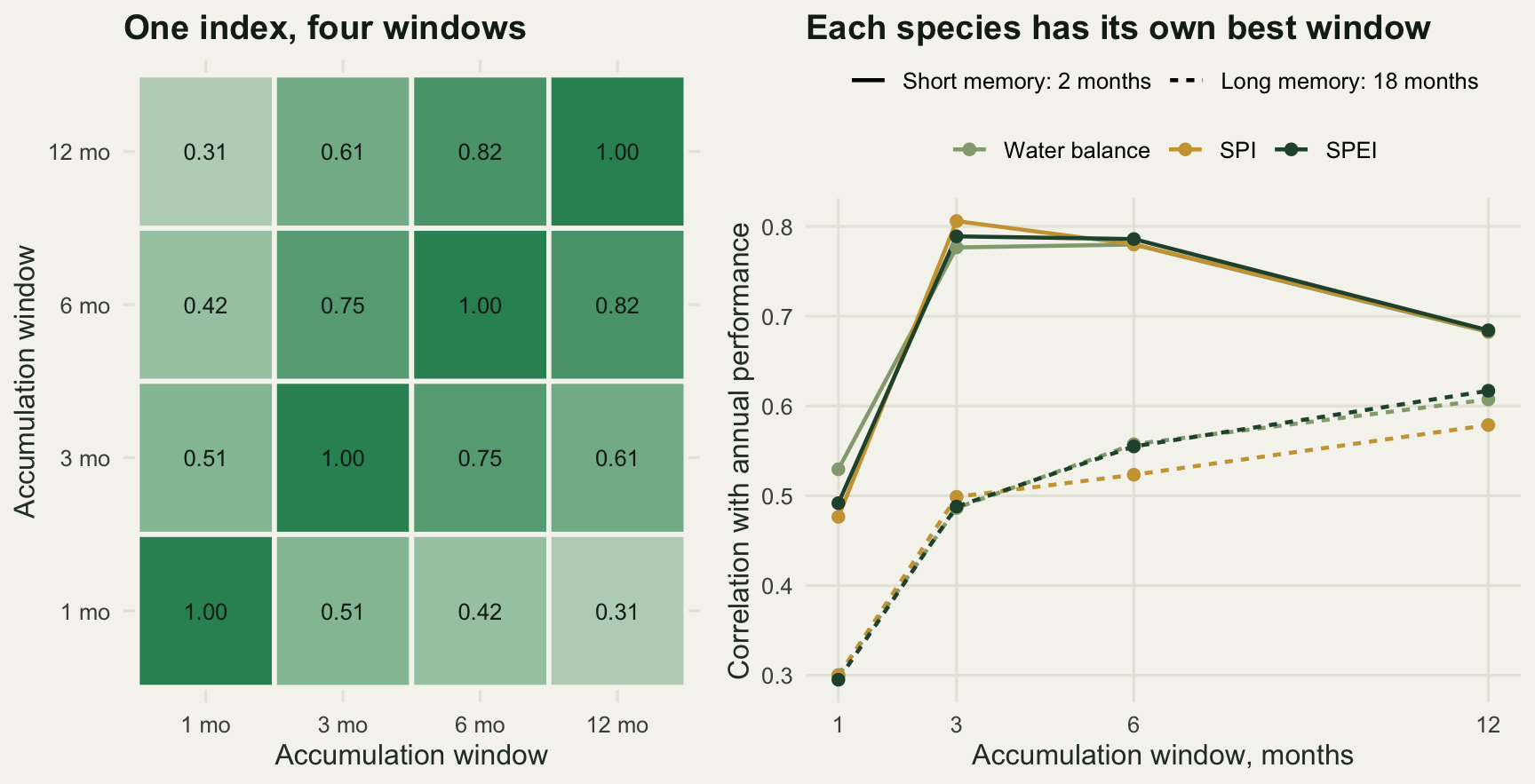
For the short memory species the SPI correlations rise from 0.477 at one month to 0.806 at three months and fall back to 0.684 at twelve. For the long memory species the SPEI correlations run the other way, from 0.295 at one month to 0.617 at twelve. The window matters more than the index: moving the short memory species from a three month window to a twelve month one costs 0.122 of correlation, while switching between the precipitation-only and the water balance version at a fixed three month window moves it by 0.017.
The winner in this realisation is the twelve month SPEI for the long memory species and the three month SPI for the short memory one. That second result was not what I expected, since the truth was generated by a bucket that subtracts evapotranspiration, so the index that also subtracts it should have won. Redrawing the observation noise 200 times, holding the weather and the index values fixed, shows what happened: the three month SPEI takes the top slot in 0.56 of draws and the six month SPEI in 0.43, while the three month SPI wins only 0.005 of them. Against the noise-free stress integral the SPEI takes the top of the ranking, 0.877 at three months and 0.875 at six against 0.857 for the three month SPI. The single realisation picked the wrong index by a margin the noise can supply. For the long memory species the twelve month SPEI wins every one of the 200 redraws on this run, and its noise-free correlation of 0.724 sits a little above 0.71 for the raw water balance and 0.681 for the SPI.
Two lessons come out of that. The window is identifiable from an ecological series, and it matters more than the choice between precipitation and water balance. And the ranking among indices at a fixed window is tight enough that a single response series can name the wrong one, as it did here, so the winner should be reported with the margin, not as a finding.
Evapotranspiration matters only when the temperature moves
The stationary record above gave almost the same answer whether demand was subtracted or not. That is not an argument for ignoring demand, it is a statement about a record whose temperature has no trend. Repeat the comparison on a record warming by 0.25 degrees a decade, and give the Thornthwaite heat index a fixed climatology from the first 30 years so that rising temperature raises demand rather than being absorbed into the normal.
set.seed(4471)
ww <- sim_weather(n_warm, warm_rate)
base_rows <- which(ww$year <= 30)
heat_base <- sum((tapply(pmax(ww$temp[base_rows], 0), ww$month[base_rows], mean) / 5)^1.514)
ptw <- pet_thorn(ww$temp, ww$month, heat_base)
ww$pet <- ptw$pet
ww$bal <- ww$precip - ww$pet
augw <- which(ww$month == anchor)[-1]
yw <- ww$year[augw]

acc_p <- accumulate(ww$precip, 12); acc_b <- accumulate(ww$bal, 12)
spi_w <- standardise(acc_p, ww$month, fit_gam, p_gam)
spei_w <- standardise(acc_b, ww$month, fit_ll, p_ll)

last20 <- augw[yw > n_warm - 20]
round(c(warm_years = n_warm, warming_per_decade = warm_rate,
        total_warming = warm_rate * (n_warm - 1) / 10,
        pet_first_decade = sum(ww$pet[ww$year <= 10]) / 10,
        pet_last_decade = sum(ww$pet[ww$year > n_warm - 10]) / 10,
        mean_annual_precip = sum(ww$precip) / n_warm), 3)
warm_years warming_per_decade total_warming pet_first_decade
120.000 0.250 2.975 543.269
pet_last_decade mean_annual_precip
673.895 504.943 round(c(cor_stationary = cor(idx_stat$spi12, idx_stat$spei12, use = "pair"),
cor_warming = cor(spi_w, spei_w, use = "pair")), 3)cor_stationary cor_warming
0.949 0.866 round(c(last20_years = length(last20),
spi_droughts = sum(spi_w[last20] < thresh),
spei_droughts = sum(spei_w[last20] < thresh),
mean_spi = mean(spi_w[last20]), mean_spei = mean(spei_w[last20])), 3) last20_years spi_droughts spei_droughts mean_spi mean_spei
20.000 4.000 7.000 -0.228 -0.836 rec_levels <- c(paste0("Stationary record, ", n_stat, " years"),
paste0("Warming ", warm_rate, " degrees per decade, ", n_warm, " years"))
warm_long <- rbind(
data.frame(year = w$year[aug[-1]], value = idx_stat$spi12[aug[-1]],
index = "SPI", record = rec_levels[1]),
data.frame(year = w$year[aug[-1]], value = idx_stat$spei12[aug[-1]],
index = "SPEI", record = rec_levels[1]),
data.frame(year = yw, value = spi_w[augw], index = "SPI", record = rec_levels[2]),
data.frame(year = yw, value = spei_w[augw], index = "SPEI", record = rec_levels[2]))
warm_long$record <- factor(warm_long$record, levels = rec_levels)
run_mean <- function(df, keys, k = 11) {
parts <- split(df, df[keys], drop = TRUE)
out <- do.call(rbind, lapply(parts, function(z) {
z <- z[order(z$year), ]
z$value <- as.numeric(stats::filter(z$value, rep(1 / k, k), sides = 2))
z[!is.na(z$value), ]
}))
out
}
warm_smooth <- run_mean(warm_long, c("index", "record"))
ggplot(warm_long, aes(year, value, colour = index)) +
geom_hline(yintercept = thresh, colour = te_pal$clay, linetype = "22", linewidth = 0.6) +
geom_line(linewidth = 0.4, alpha = 0.4) +
geom_line(data = warm_smooth, linewidth = 1.2) +
facet_wrap(~record) +
scale_colour_manual(values = c(SPI = te_pal$gold, SPEI = te_pal$forest), name = NULL) +
scale_x_continuous(breaks = seq(0, 150, by = 50),
expand = expansion(mult = c(0.03, 0.03))) +
labs(x = "Year of record, shared by both panels",
y = "Index in August, 12 month window",
title = "Two indices that agree until it warms") +
theme_te() +
theme(legend.position = "top",
strip.text = element_text(colour = te_pal$ink, face = "bold"),
plot.margin = margin(5.5, 14, 5.5, 5.5))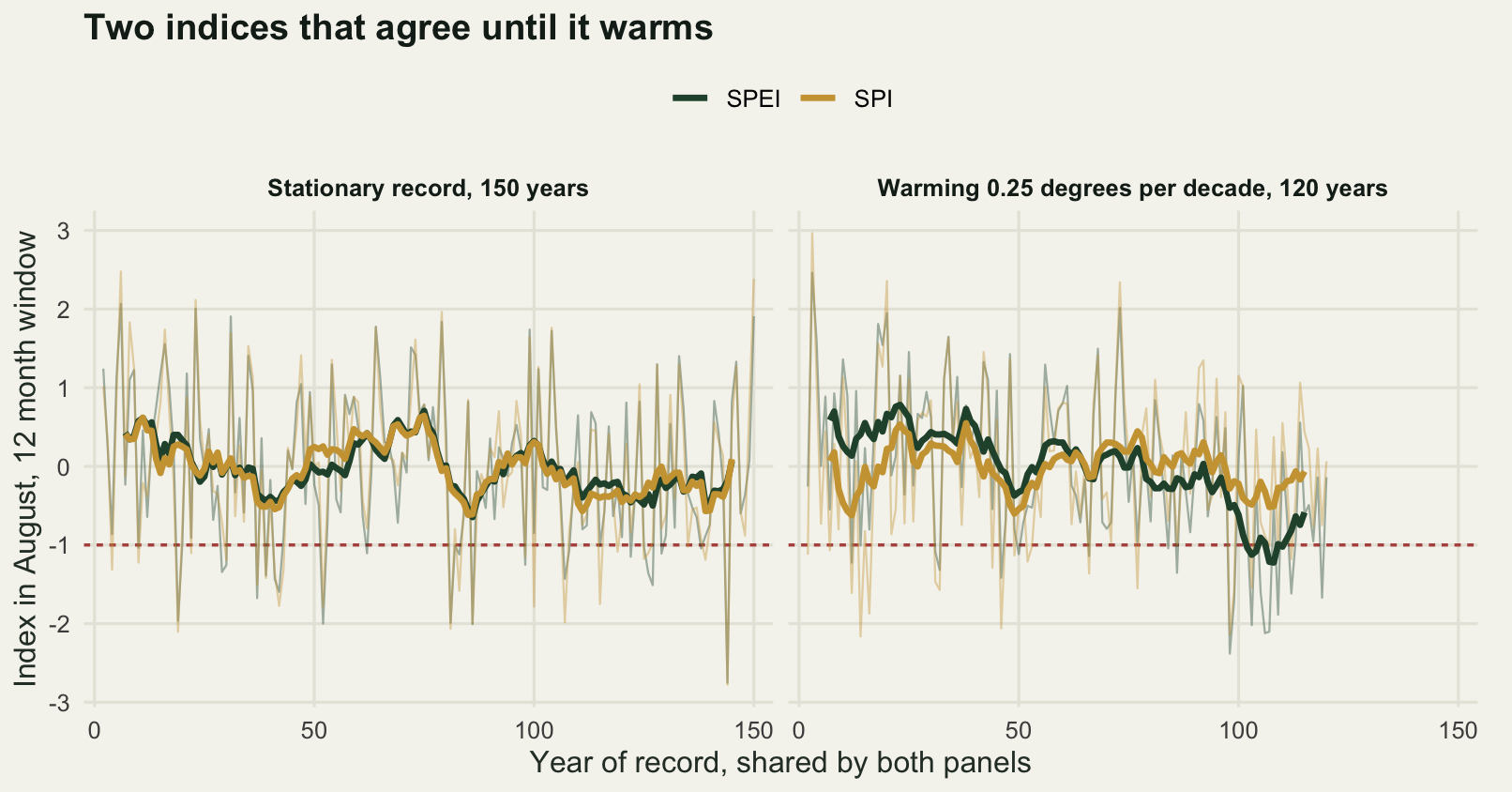
Over 120 years the record warms by 2.975 degrees. Annual potential evapotranspiration rises from 543.269 mm in the first decade to 673.895 mm in the last, an increase larger than a quarter of the mean annual precipitation of 504.943 mm, while precipitation itself has no trend at all by construction. The correlation between the twelve month SPI and the twelve month SPEI is 0.949 in the stationary record and 0.866 in the warming one.
In the last two decades of the warming record the SPI flags 4 Augusts as drought and the SPEI flags 7. The means are more telling than the counts: the mean SPI over those 20 years is -0.228, consistent with an unchanged rainfall regime, while the mean SPEI is -0.836, shifted towards the drought threshold. The precipitation-only index says nothing has happened, because from its point of view nothing has. It is not wrong. It is answering a question about rainfall while the plants are living through a question about water.
The baseline period moves the number without moving the ranking
A standardised index is standardised against something. Change the reference years and the same weather receives a different index value. Start on the stationary record, where the choice should be harmless, and compare a baseline of the first 30 years with one of the first 100.
ay <- aug[-1]
acc12 <- accumulate(w$precip, 12)
spi30 <- standardise(acc12, w$month, fit_gam, p_gam, ref = which(w$year <= 31))[ay]
spi100 <- standardise(acc12, w$month, fit_gam, p_gam, ref = which(w$year <= 100))[ay]
driest <- which.min(spi100)
round(c(baseline_short = 30, baseline_long = 100,
        driest_year = w$year[ay][driest],
        spi_short_baseline = spi30[driest], spi_long_baseline = spi100[driest]), 3)
baseline_short baseline_long driest_year spi_short_baseline
30.000 100.000 144.000 -2.768
spi_long_baseline
-2.869 round(c(mean_abs_diff = mean(abs(spi30 - spi100)),
max_abs_diff = max(abs(spi30 - spi100)),
pearson = cor(spi30, spi100),
spearman = cor(spi30, spi100, method = "spearman"),
droughts_short_baseline = sum(spi30 < thresh),
droughts_long_baseline = sum(spi100 < thresh)), 4) mean_abs_diff max_abs_diff pearson
0.1449 0.3585 1.0000
spearman droughts_short_baseline droughts_long_baseline
1.0000 27.0000 26.0000 The driest August in the record is year 144. Standardised against the first 30 years its SPI is -2.768; against the first 100 years it is -2.869. Across all years the mean absolute difference between the two versions is 0.1449 and the largest is 0.3585. The rank correlation is exactly 1, as the monotone construction guarantees, and the ordinary correlation rounds to 1 as well. Yet the drought year count changes, from 27 under the short baseline to 26 under the long one, because a threshold cuts a continuous variable and any shift moves some years across the cut. On a stationary record the baseline is a nuisance of about a tenth of an index unit.
On a warming record it stops being a nuisance. Take the twelve month August water balance and standardise it two ways: once against a fixed baseline of the first 30 available years, and once against a moving baseline of the previous 30 years, refitted for every year.
bal_aug <- acc_b[augw]
fix_par <- fit_ll(bal_aug[1:30])
spei_fix <- qnorm(p_ll(bal_aug, fix_par))
spei_mov <- rep(NA_real_, length(bal_aug))
for (i in 31:length(bal_aug)) {
  spei_mov[i] <- qnorm(p_ll(bal_aug[i], fit_ll(bal_aug[(i - 30):(i - 1)])))
}

fin <- which(yw > n_warm - 10)
dec <- yw / 10
slope_of <- function(v, d) {
  ok <- !is.na(v); m <- lm(v[ok] ~ d[ok])
  c(per_decade = as.numeric(coef(m)[2]), p_value = summary(m)$coefficients[2, 4])
}
round(c(final_decade_years = length(fin),
        droughts_fixed_baseline = sum(spei_fix[fin] < thresh),
        droughts_moving_baseline = sum(spei_mov[fin] < thresh),
        mean_fixed = mean(spei_fix[fin]), mean_moving = mean(spei_mov[fin])), 3)
final_decade_years droughts_fixed_baseline droughts_moving_baseline
10.000 7.000 2.000
mean_fixed mean_moving
-1.272 -0.118 round(c(balance_first_decade_mm = mean(bal_aug[1:10]),
balance_final_decade_mm = mean(bal_aug[fin])), 3)balance_first_decade_mm balance_final_decade_mm
-7.719 -184.230 sl_tab <- rbind(water_balance = slope_of(bal_aug, dec),
spei_fixed = slope_of(spei_fix, dec),
spei_moving = slope_of(spei_mov, dec))
print(signif(sl_tab, 4)) per_decade p_value
water_balance -15.36000 2.960e-07
spei_fixed -0.14320 2.564e-07
spei_moving -0.02196 6.002e-01print(round(sl_tab[, "p_value"], 4))water_balance spei_fixed spei_moving
0.0000 0.0000 0.6002 bp <- c("12 month water balance in August (mm)", "Standardised index")
base_long <- rbind(
data.frame(year = yw, value = bal_aug, series = "Water balance", panel = bp[1]),
data.frame(year = yw, value = spei_fix, series = "Fixed 30 year baseline", panel = bp[2]),
data.frame(year = yw, value = spei_mov, series = "Moving 30 year baseline", panel = bp[2]))
base_long$panel <- factor(base_long$panel, levels = bp)
base_long <- base_long[!is.na(base_long$value), ]
flag <- base_long[base_long$panel == bp[2] & base_long$value < thresh, ]
cutl <- data.frame(yv = thresh, panel = factor(bp[2], levels = bp))
band <- data.frame(xmin = n_warm - 9.5, xmax = n_warm + 0.5)
base_smooth <- run_mean(base_long, c("series", "panel"))
ggplot(base_long, aes(year, value, colour = series)) +
geom_rect(data = band, aes(xmin = xmin, xmax = xmax, ymin = -Inf, ymax = Inf),
inherit.aes = FALSE, fill = te_pal$sage, alpha = 0.25) +
geom_hline(data = cutl, aes(yintercept = yv), colour = te_pal$clay,
linetype = "22", linewidth = 0.6) +
geom_line(linewidth = 0.4, alpha = 0.45) +
geom_line(data = base_smooth, linewidth = 1.2) +
geom_point(data = flag, size = 1.6) +
facet_wrap(~panel, ncol = 1, scales = "free_y") +
scale_colour_manual(values = c("Water balance" = te_pal$sage,
"Fixed 30 year baseline" = te_pal$forest,
"Moving 30 year baseline" = te_pal$gold), name = NULL) +
labs(x = "Year of record", y = NULL,
title = "A moving baseline hides a falling water balance") +
theme_te() +
theme(legend.position = "top",
strip.text = element_text(colour = te_pal$ink, face = "bold"))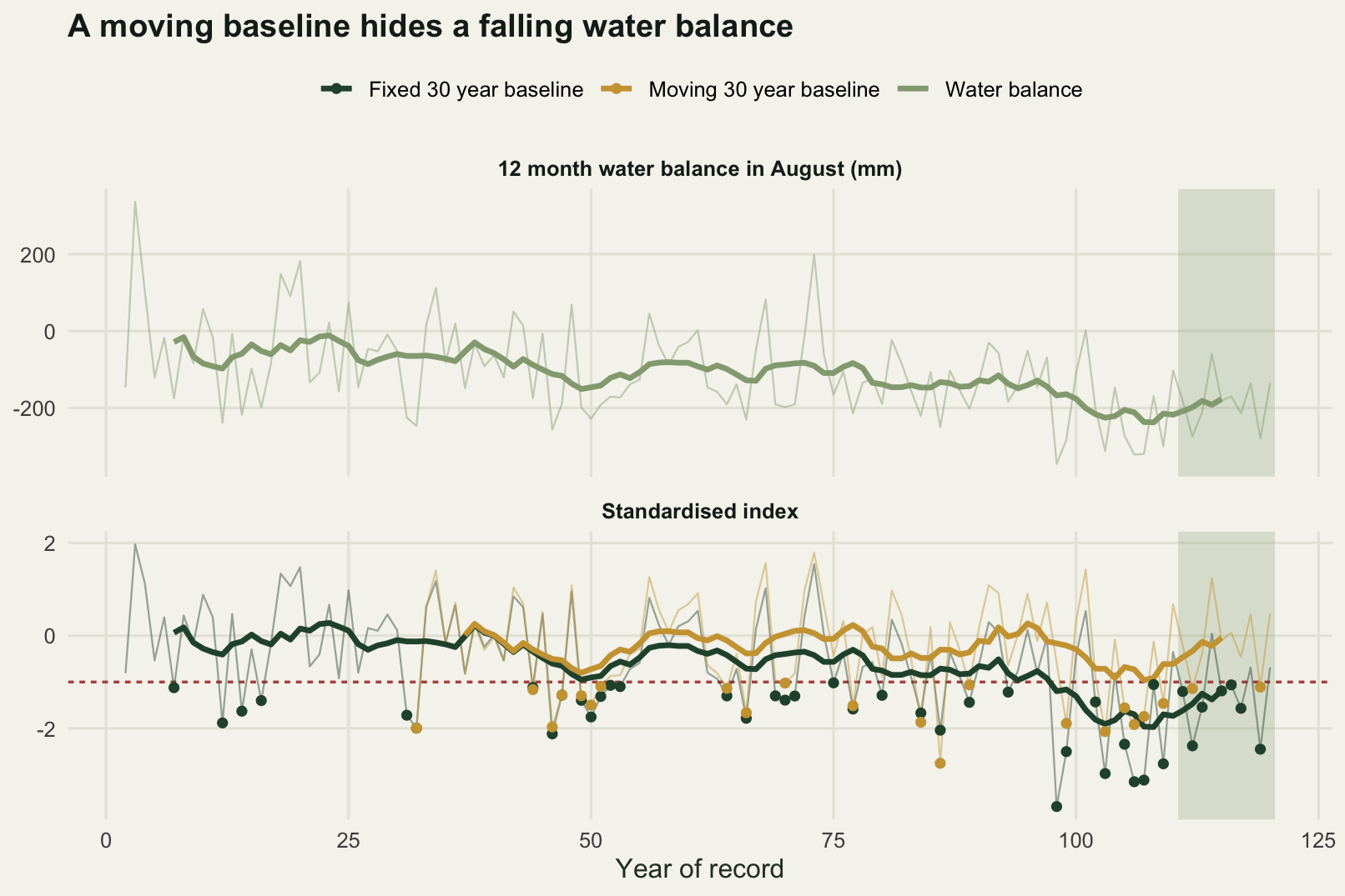
In the final decade the fixed baseline calls 7 of the 10 years drought and the moving baseline calls 2. Their mean index values in that decade are -1.272 and -0.118. Underneath both, the water balance itself has fallen from a mean of -7.719 mm over the first decade to -184.23 mm over the last, a slope of -15.36 mm per decade with a p-value of 2.96 times ten to the minus seven. The fixed baseline index inherits that trend, at -0.1432 index units per decade with the same significance. The moving baseline index has a slope of -0.02196 per decade and a p-value of 0.6002: no trend in drought at all.
Neither number is a mistake. A standardised index with a moving baseline measures departure from recent conditions, and by the end of the record recent conditions are dry, so a year that would have been extraordinary in the first decade is now ordinary and receives a value near zero. That is exactly what you want if the question is about anomalies relative to what the system is currently adapted to, and exactly what you do not want if the question is whether water availability is declining. The choice is a scientific one that arrives disguised as a preprocessing detail, and a paper reporting no trend in drought frequency over a warming century has not reported a fact about water until it says which baseline produced the sentence.
What the index cannot tell you
The honest limit is in the results already, so it can be stated as a measurement rather than as a caution. Two species lived through exactly the same weather. One integrates water stress over two months and is best described by a three month standardised index, which recovers a correlation of 0.877 with its underlying stress. The other integrates over 18 months, is best described by a twelve month index, and its best available correlation is 0.724. Feed the long memory species the index that suits the short memory one and the correlation drops to 0.56; feed the short memory species the twelve month index and it drops to 0.755. There is no drought index in this post, and none in the literature, that is simultaneously the right one for both.
pick <- function(row, tag) {
  v <- noise_free[row, ]; nm <- names(v)
  sub <- v[grepl(paste0("^", tag), nm)]
  c(best = round(max(sub), 3), window = windows[which.max(sub)])
}
cross <- c(A_at_12_month = noise_free["A", "spei12"],
           B_at_3_month = noise_free["B", "spei3"])
print(round(rbind(A = pick("A", "spei"), B = pick("B", "spei")), 3))
best window
A 0.877 3
B 0.724 12round(cross, 3)A_at_12_month B_at_3_month
0.755 0.560 round(c(loss_A_wrong_window = noise_free["A", "spei3"] - noise_free["A", "spei12"],
loss_B_wrong_window = noise_free["B", "spei12"] - noise_free["B", "spei3"]), 3)loss_A_wrong_window loss_B_wrong_window
0.122 0.164 Three further limits are worth naming because the simulation cannot measure them and a real analysis will meet all three.
The weather generator here never produces a month with zero rainfall, because the gamma distribution is continuous and positive. Real records in dry regions produce them in quantity, and the gamma has no density at zero, so the standard fix is a mixture: estimate the probability of a dry month, fit the gamma to the wet ones, and splice the two together in the probability transform. Skip that step and the index in an arid month is not defined.
Thornthwaite’s formula knows only temperature. It has no radiation, no vapour pressure deficit and no wind, so it converts a warm year into a thirsty year by construction. Since the warming experiment above raised temperature and nothing else, the size of the divergence between the two indices is partly a property of the formula. A Penman-Monteith demand would move less for the same warming if humidity rose with it, and the water balance panel would fall less steeply. The direction of the result stands; the slope of -15.36 mm per decade does not transfer.
And the whole post rests on one weather realisation and one bucket. The bucket has a single capacity of 100 mm, no rooting depth, no runoff and no snow, so it says nothing about a species whose water comes from a water table or from snowmelt timing. The correct reading of the results is comparative: the window is worth more than the index, the baseline is worth more than either under a trend, and the ranking among indices can sit inside the noise.
Where to go next
The natural next step is to stop choosing a window by hand. A sliding window search over an ecological response finds the accumulation period the organism responds to, at the cost of a multiple testing problem that has to be handled explicitly, and climate window analysis in R sets that up. Once a window is selected, the checks in checking a climate window analysis apply directly to a drought index, because a drought variable chosen from twelve candidates carries the same inflation as a temperature window chosen from fifty. If the response of interest is timing rather than growth, degree days and thermal time in R builds the temperature side of the same problem with the same care about accumulation.
References
McKee TB, Doesken NJ, Kleist J 1993 Proceedings of the Eighth Conference on Applied Climatology. American Meteorological Society, Boston:179-184 (no DOI)
Vicente-Serrano SM, Begueria S, Lopez-Moreno JI 2010 Journal of Climate 23(7):1696-1718 (10.1175/2009JCLI2909.1)
Thornthwaite CW 1948 Geographical Review 38(1):55-94 (10.2307/210739)
Slette IJ, Post AK, Awad M, Even T, Punzalan A, Williams S, Smith MD, Knapp AK 2019 Global Change Biology 25(10):3193-3200 (10.1111/gcb.14747)
Begueria S, Vicente-Serrano SM, Reig F, Latorre B 2014 International Journal of Climatology 34(10):3001-3023 (10.1002/joc.3887)