library(ggplot2)
library(patchwork)

te_paper  <- "#f5f4ee"
te_ink    <- "#16241d"
te_body   <- "#2c3a31"
te_forest <- "#275139"
te_rust   <- "#b5534e"
te_gold   <- "#c9b458"
te_line   <- "#dad9ca"

theme_datasheet <- function() {
  theme_minimal(base_size = 12) +
    theme(plot.background  = element_rect(fill = te_paper, colour = NA),
          panel.background = element_rect(fill = te_paper, colour = NA),
          panel.grid.major = element_line(colour = te_line, linewidth = 0.3),
          panel.grid.minor = element_blank(),
          text             = element_text(colour = te_body),
          plot.title       = element_text(colour = te_ink, face = "bold"),
          plot.subtitle    = element_text(colour = te_body),
          axis.text        = element_text(colour = te_body))
}Heatwave counts: persistence, rule order, warming
R
climate
extremes
time series
simulation
ecology tutorial
How many heatwaves a year depends on persistence and on the order of the duration and gap rules. Simulating the Hobday marine heatwave definition in R.
A temperature logger has sat in a seagrass meadow for forty years, and the monitoring report now carries a line that reads “marine heatwaves per year”. The meadow lost shoots after two long warm spells, so the line matters: managers compare it between sites, and between decades at the same site. For marine heatwaves the definition behind it is usually the one Hobday and colleagues proposed in 2016. A day is hot when its temperature is above the 90th percentile for that day of the year, taken from a 30-year baseline; a heatwave is at least five hot days in a row; and two heatwaves separated by a gap of two days or less are joined into one.
That definition is an estimator, and its output is a count. This post measures what the count responds to. The first finding is that at an unchanged ten per cent of hot days the number of heatwaves is set by how persistent the daily anomalies are, and that reading the two rules in the wrong order changes it several times over. The second is what happens under warming against a fixed baseline: the count rises, peaks and falls while hot days keep climbing, and sites with different persistence swap places on the way. A stationary record with the threshold lowered step by step, and no warming at all, shows the same peak and the same swap, so both belong to the share of days above the threshold; warming moves a site along that curve, and where the share climbs steeply inside the counted decade the count sits below it. Most of this is a demonstration of known material. The definition, including the order of its two rules, is Hobday and colleagues’ own: their gap rule joins only events that are themselves at least five days long, and both the heatwaveR package (Schlegel and Smit 2018) and the original Python module code it that way. The tension between a fixed baseline and a warming record is the one Jacox (2019) set out. What is measured here is how large the effects are on a simple simulated series.
Three posts on this site sit nearby and do different jobs. Peaks over threshold and the GPD opens its declustering section with “A heatwave is several hot days in a row, not one”, but it declusters exceedances in order to fit a tail distribution; the cluster there is a nuisance for the likelihood, not the quantity being reported. Drought indices for ecologists already shows that the baseline period moves an index value without moving the ranking of years, so the baseline gets only a short section here. Reset time and the double-counted hot day is about how a single daily maximum is recorded in the first place; this post takes the daily values as given and asks how they are strung into events.
Two readings of the same two rules
Hobday and colleagues (2016) join a gap of two days or less only between events that already last five days or more; their worked example is five warm days, two cool days and six warm days, which make one 13-day event. So the minimum comes first: find runs of hot days, keep only runs of at least five days, and then join kept runs whose gap is two days or less. This is also the order coded in heatwaveR (Schlegel and Smit 2018). A detector written from the short summary “five days, gaps of two joined” can easily fill the gaps first instead, which turns two short hot runs into one long run, and only then apply the five-day minimum. That merge-first reading is a misreading of the definition, not a published alternative; it is simulated here because the size of the error is the useful number. Both detectors take a logical vector of hot days.
min_len_hw <- 5    # minimum heatwave length, days
max_gap_hw <- 2    # longest gap that still joins two heatwaves, days

# Hobday order: drop runs shorter than min_len, then join the survivors
hobday_events <- function(hot, min_len = min_len_hw, max_gap = max_gap_hw) {
  r_hot <- rle(hot)
  e_run <- cumsum(r_hot$lengths)
  s_run <- e_run - r_hot$lengths + 1
  keep  <- which(r_hot$values & r_hot$lengths >= min_len)
  if (length(keep) == 0) return(list(n = 0L, start = integer(0), end = integer(0)))
  s_run <- s_run[keep]
  e_run <- e_run[keep]
  if (length(s_run) > 1 && max_gap > 0) {
    opens <- c(TRUE, s_run[-1] - e_run[-length(e_run)] - 1 > max_gap)
    s_run <- s_run[opens]
    e_run <- e_run[c(opens[-1], TRUE)]
  }
  list(n = length(s_run), start = s_run, end = e_run)
}

# merge-first order: fill short cool gaps, then drop runs shorter than min_len
merge_first_events <- function(hot, min_len = min_len_hw, max_gap = max_gap_hw) {
  r_hot <- rle(hot)
  n_run <- length(r_hot$values)
  fill  <- !r_hot$values & r_hot$lengths <= max_gap
  fill[c(1, n_run)] <- FALSE
  r_hot$values[fill] <- TRUE
  r_two <- rle(inverse.rle(r_hot))
  e_run <- cumsum(r_two$lengths)
  s_run <- e_run - r_two$lengths + 1
  keep  <- which(r_two$values & r_two$lengths >= min_len)
  list(n = length(keep), start = s_run[keep], end = e_run[keep])
}

toy_hot <- as.logical(c(0, 1, 1, 1, 0, 1, 1, 1, 0, 0, 0,
                        1, 1, 1, 1, 1, 0, 1, 0))
toy_hob <- hobday_events(toy_hot)
toy_mf  <- merge_first_events(toy_hot)
toy_hob_len <- toy_hob$end - toy_hob$start + 1
toy_mf_len  <- toy_mf$end - toy_mf$start + 1
A short string makes the difference concrete. It holds a run of three hot days, one cool day, three more hot days, three cool days, a run of five hot days, one cool day and a single hot day. The Hobday order finds 1 heatwave of 5 days: neither three-day run reaches the minimum, and the lone hot day after the five-day run is not a heatwave that could be joined. The merge-first order finds 2 heatwaves, of 7 and 7 days, because the single cool days were filled before the minimum was checked. The minimum in the merge-first reading is a minimum on the span of the event, not on any run of consecutive hot days inside it.
The series used throughout is a daily record of 40 years: a seasonal sine wave plus a first-order autoregressive anomaly with unit variance and lag-one correlation phi, plus, later, a linear warming trend. Everything is in units of the anomaly standard deviation, so a trend of 0.02 means two hundredths of a daily standard deviation per year. The threshold follows the heatwaveR defaults: the 90th percentile of all baseline values within five days either side of each day of the year, then a 31-day circular moving average. The climatology used for intensity is built the same way from the mean.
n_year     <- 40
n_doy      <- 365
seas_amp   <- 3            # seasonal amplitude, anomaly SD units
half_win   <- 5            # days either side of the day of year
smooth_len <- 31           # moving average for threshold and climatology
pct_hot    <- 0.9
base_years <- 1:30         # fixed baseline
last_years <- 31:40        # decade in which everything is counted

year_id  <- rep(seq_len(n_year), each = n_doy)
doy_id   <- rep(seq_len(n_doy), n_year)
seasonal <- seas_amp * sin(2 * pi * doy_id / n_doy)

ar1_series <- function(n, phi) {
  as.numeric(stats::filter(rnorm(n, 0, sqrt(1 - phi^2)), phi,
                           method = "recursive", init = rnorm(1)))
}

win_idx <- outer(seq_len(n_doy), -half_win:half_win,
                 function(d, o) ((d + o - 1) %% n_doy) + 1)
circ_smooth <- function(v, width) {
  as.numeric(stats::filter(v, rep(1 / width, width), circular = TRUE))
}

# threshold and climatology from a years x days matrix, vectorised:
# one order() call sorts every day-of-year window at once
doy_climatology <- function(x_mat) {
  n_b    <- nrow(x_mat)
  n_pool <- n_b * ncol(win_idx)
  pooled <- as.vector(x_mat[, as.vector(t(win_idx)), drop = FALSE])
  grp    <- rep(rep(seq_len(n_doy), each = ncol(win_idx)), each = n_b)
  sorted <- matrix(pooled[order(grp, pooled)], nrow = n_doy, byrow = TRUE)
  h_pos  <- (n_pool - 1) * pct_hot + 1
  lo     <- floor(h_pos)
  thr    <- sorted[, lo] + (h_pos - lo) * (sorted[, lo + 1] - sorted[, lo])
  list(thresh = circ_smooth(thr, smooth_len),
       clim   = circ_smooth(rowMeans(sorted), smooth_len))
}

set.seed(20160)
check_mat <- matrix(rnorm(30 * n_doy), 30, n_doy)
check_thr <- sapply(seq_len(n_doy), function(d)
  quantile(check_mat[, win_idx[d, ]], pct_hot, names = FALSE))
check_gap <- max(abs(circ_smooth(check_thr, smooth_len) -
                     doy_climatology(check_mat)$thresh))
The vectorised threshold agrees with quantile() applied day by day to within 4.44e-16, which is rounding error.
Ten per cent of the days, very different numbers of heatwaves
To separate the rules from the threshold, this section uses the true 90th percentile of the anomaly and no seasonal cycle, so exactly ten per cent of days are hot in expectation whatever the persistence. Each value of phi gets one long stationary record cut into decades, and the Monte Carlo standard error of the yearly count comes from the spread among decades.
phi_grid  <- c(0.2, 0.3, 0.4, 0.5, 0.6, 0.7, 0.8, 0.9, 0.95)
n_decade  <- 300
dec_len   <- 3650
thr_true  <- qnorm(pct_hot)

per_decade <- function(ev, n_dec) {
  tabulate((ev$start - 1) %/% dec_len + 1, nbins = n_dec)
}

set.seed(20162)
stat_hot <- list()
stat_tab <- do.call(rbind, lapply(phi_grid, function(phi) {
  hot <- ar1_series(n_decade * dec_len, phi) > thr_true
  stat_hot[[as.character(phi)]] <<- hot
  ev_h <- hobday_events(hot)
  ev_m <- merge_first_events(hot)
  c_h  <- per_decade(ev_h, n_decade) / 10
  c_m  <- per_decade(ev_m, n_decade) / 10
  d_hot <- tabulate((which(hot) - 1) %/% dec_len + 1, nbins = n_decade) / 10
  data.frame(phi = phi, hot_days = mean(d_hot),
             hob = mean(c_h), hob_se = sd(c_h) / sqrt(n_decade),
             mf = mean(c_m), mf_se = sd(c_m) / sqrt(n_decade),
             hob_dur = mean(ev_h$end - ev_h$start + 1),
             mf_dur = mean(ev_m$end - ev_m$start + 1))
}))
stat_tab$ratio <- stat_tab$mf / stat_tab$hob

st <- function(phi, col) stat_tab[[col]][stat_tab$phi == phi]
hot_range <- range(stat_tab$hot_days)
ratio_05  <- st(0.5, "ratio")
ratio_95  <- st(0.95, "ratio")
hob_span  <- max(stat_tab$hob) / st(0.5, "hob")
mf_span   <- max(stat_tab$mf) / min(stat_tab$mf)
phi_mf_max <- stat_tab$phi[which.max(stat_tab$mf)]
phi_hob_max <- stat_tab$phi[which.max(stat_tab$hob)]
Across the whole grid the hot days per year stay between 36.3 and 36.8, against the nominal 36.5. The heatwave counts do not stay put. Under the Hobday order a series with phi 0.5 gives 0.31 heatwaves per year (Monte Carlo SE 0.01), phi 0.8 gives 1.77 (SE 0.02) and phi 0.95 gives 2.05 (SE 0.03). Under the merge-first order the same three records give 2.10, 3.15 and 2.51.
At phi 0.5 the merge-first detector reports 6.7 times as many heatwaves as the Hobday detector on identical data. At phi 0.95 the ratio is 1.22, because hot runs in a very persistent series are already long and the short gaps decide far fewer events. The two orders also disagree about what persistence does. Under the Hobday order the count keeps rising with phi until it reaches 2.23 at phi 0.9, 7.1 times the phi 0.5 value, and then drops slightly. Under merge-first it peaks at phi 0.8 and the whole grid spans only a factor of 2.1. Mean event length under the Hobday order grows from 5.5 days at phi 0.5 to 13.0 days at phi 0.95.
The mechanism is plain once it is drawn. With little persistence a ten per cent exceedance rate produces many short hot runs; very few reach five days, so the Hobday count is small, while merge-first stitches pairs of three- and four-day runs into five-day events. With strong persistence the hot days come already bundled in long runs, and bundling them further reduces the count rather than raising it.
pers_long <- rbind(
  data.frame(phi = stat_tab$phi, events = stat_tab$hob, se = stat_tab$hob_se,
             order = "Hobday order (minimum, then join)"),
  data.frame(phi = stat_tab$phi, events = stat_tab$mf, se = stat_tab$mf_se,
             order = "merge-first order (join, then minimum)"))

ggplot(pers_long, aes(phi, events, colour = order)) +
  geom_errorbar(aes(ymin = events - 2 * se, ymax = events + 2 * se),
                width = 0.012, linewidth = 0.5) +
  geom_line(linewidth = 0.9) +
  geom_point(size = 2.2) +
  scale_colour_manual(values = c(te_forest, te_gold), name = NULL) +
  scale_y_continuous(limits = c(0, NA)) +
  labs(x = "lag-one autocorrelation of the daily anomaly (phi)",
       y = "heatwaves per year",
       title = "One exceedance rate, many heatwave counts",
       subtitle = "hot days fixed at ten per cent; bars: two Monte Carlo SEs") +
  theme_datasheet() +
  theme(legend.position = "bottom") +
  guides(colour = guide_legend(nrow = 2))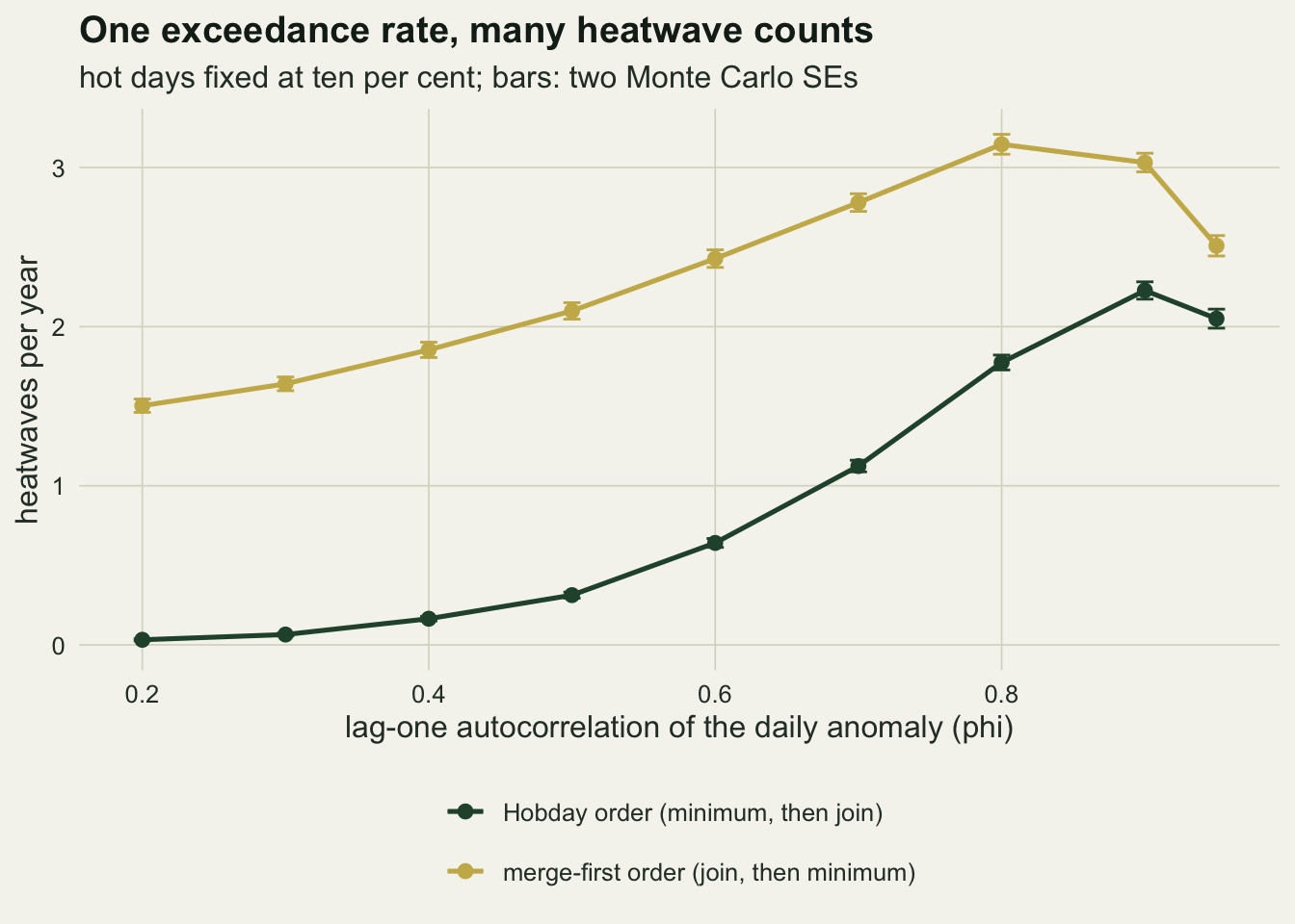
The two numbers in the rule matter as much as their order. The table uses the same three stationary records and varies the minimum length and the gap. With no gap joining the two orders are the same detector, so their columns agree in the rows with a gap of zero.
rule_phi <- c(0.5, 0.8, 0.95)
rule_set <- expand.grid(min_len = c(3, 5), max_gap = c(0, 2))
rule_tab <- do.call(rbind, lapply(seq_len(nrow(rule_set)), function(i) {
  ml <- rule_set$min_len[i]
  mg <- rule_set$max_gap[i]
  vals <- vapply(rule_phi, function(phi) {
    hot <- stat_hot[[as.character(phi)]]
    c(hobday_events(hot, ml, mg)$n, merge_first_events(hot, ml, mg)$n) /
      (n_decade * 10)
  }, numeric(2))
  data.frame(min_len = ml, max_gap = mg,
             hob_05 = vals[1, 1], mf_05 = vals[2, 1],
             hob_08 = vals[1, 2], mf_08 = vals[2, 2],
             hob_95 = vals[1, 3], mf_95 = vals[2, 3])
}))
rule_show <- rule_tab
names(rule_show) <- c("minimum (days)", "gap (days)",
                      "phi 0.5 Hobday", "phi 0.5 merge-first",
                      "phi 0.8 Hobday", "phi 0.8 merge-first",
                      "phi 0.95 Hobday", "phi 0.95 merge-first")
knitr::kable(rule_show, digits = 2, row.names = FALSE)| minimum (days) | gap (days) | phi 0.5 Hobday | phi 0.5 merge-first | phi 0.8 Hobday | phi 0.8 merge-first | phi 0.95 Hobday | phi 0.95 merge-first |
|---|---|---|---|---|---|---|---|
| 3 | 0 | 2.69 | 2.69 | 4.60 | 4.60 | 3.60 | 3.60 |
| 5 | 0 | 0.31 | 0.31 | 1.83 | 1.83 | 2.28 | 2.28 |
| 3 | 2 | 2.63 | 5.62 | 4.26 | 5.57 | 3.04 | 3.38 |
| 5 | 2 | 0.31 | 2.10 | 1.77 | 3.15 | 2.05 | 2.51 |
rt <- function(ml, mg, col) rule_tab[[col]][rule_tab$min_len == ml & rule_tab$max_gap == mg]
min3_vs_5 <- rt(3, 2, "hob_05") / rt(5, 2, "hob_05")
Relaxing the minimum from five days to three multiplies the Hobday count at phi 0.5 by 8.4, from 0.31 to 2.63 per year. Under the Hobday order the gap rule can only merge events, so it lowers the count: at phi 0.8 from 1.83 with no joining to 1.77. Under merge-first the same gap rule raises the count at phi 0.5, from 0.31 to 2.10, because filling a gap can create an event that did not exist. A methods section that says only “five days, gaps of two joined” leaves room for exactly this misreading, and the table shows what it costs; quoting Hobday and colleagues’ full gap sentence, or naming the implementation, removes it.
Warming against a fixed baseline
Now the full pipeline: seasonal cycle, estimated day-of-year threshold from years 1 to 30, and a linear trend over all 40 years, with heatwaves counted in years 31 to 40. Everything in this section uses the Hobday order unless the merge-first count is named. Each combination of persistence and trend gets 100 independent records.
trend_grid <- c(0, 0.02, 0.04, 0.06, 0.08, 0.10, 0.12, 0.16, 0.20, 0.25, 0.30)
phi_warm   <- c(0.5, 0.8, 0.95)
n_rep      <- 100
in_last    <- year_id %in% last_years
base_rows  <- base_years
recent_rows <- 21:30

count_last <- function(x, cl) {
  hot  <- x > rep(cl$thresh, n_year)
  ev   <- hobday_events(hot[in_last])
  ev_m <- merge_first_events(hot[in_last])
  ev_day <- logical(sum(in_last))
  for (i in seq_len(ev$n)) ev_day[ev$start[i]:ev$end[i]] <- TRUE
  excess <- (x - rep(cl$clim, n_year))[in_last]
  c(days = sum(hot[in_last]) / 10, events = ev$n / 10, mf = ev_m$n / 10,
    dur = if (ev$n > 0) mean(ev$end - ev$start + 1) else NA,
    ev_days = sum(ev_day) / 10, cum_int = sum(excess[ev_day]) / 10)
}

warm_run <- function(phi, trend) {
  x_all <- seasonal + ar1_series(n_year * n_doy, phi) + trend * (year_id - 1)
  x_mat <- matrix(x_all, n_year, n_doy, byrow = TRUE)
  out   <- count_last(x_all, doy_climatology(x_mat[base_rows, ]))
  if (phi == 0.8) {
    # short recent baseline, years 21 to 30
    rec <- count_last(x_all, doy_climatology(x_mat[recent_rows, ]))
    # shifting baseline: remove the linear trend fitted to annual means
    ann   <- rowMeans(x_mat)
    slope <- coef(lm(ann ~ seq_len(n_year)))[2]
    x_det <- x_all - slope * (year_id - 1)
    det_out <- count_last(x_det, doy_climatology(
      matrix(x_det, n_year, n_doy, byrow = TRUE)[base_rows, ]))
    out <- c(out, rec_days = rec[["days"]], rec_events = rec[["events"]],
             det_days = det_out[["days"]], det_events = det_out[["events"]])
  }
  out
}

set.seed(20163)
t_start <- proc.time()[["elapsed"]]
warm_tab <- do.call(rbind, lapply(phi_warm, function(phi) {
  do.call(rbind, lapply(trend_grid, function(tr) {
    reps <- replicate(n_rep, warm_run(phi, tr))
    data.frame(phi = phi, trend = tr,
               days = mean(reps["days", ]), events = mean(reps["events", ]),
               events_se = sd(reps["events", ]) / sqrt(n_rep),
               mf = mean(reps["mf", ]),
               dur = mean(reps["ev_days", ]) / mean(reps["events", ]),
               ev_days = mean(reps["ev_days", ]),
               cum_int = mean(reps["cum_int", ]),
               rec_days = if (phi == 0.8) mean(reps["rec_days", ]) else NA,
               rec_events = if (phi == 0.8) mean(reps["rec_events", ]) else NA,
               det_days = if (phi == 0.8) mean(reps["det_days", ]) else NA,
               det_events = if (phi == 0.8) mean(reps["det_events", ]) else NA)
  }))
}))
warm_secs <- proc.time()[["elapsed"]] - t_start

wt <- function(phi, tr, col) warm_tab[[col]][warm_tab$phi == phi & abs(warm_tab$trend - tr) < 1e-9]
peak_of <- function(phi) {
  sub_tab <- warm_tab[warm_tab$phi == phi, ]
  sub_tab[which.max(sub_tab$events), ]
}
pk05 <- peak_of(0.5); pk08 <- peak_of(0.8); pk95 <- peak_of(0.95)
max_se <- max(warm_tab$events_se)
shift_sd <- trend_grid * (mean(last_years) - mean(base_years))
# how far the grid neighbours of each peak sit below it
nb_gap <- function(phi) {
  ev <- warm_tab$events[warm_tab$phi == phi]
  i_pk <- which.max(ev)
  nb <- ev[intersect(c(i_pk - 1, i_pk + 1), seq_along(ev))]
  min(ev[i_pk] - nb)
}
# the same gap in Monte Carlo SEs of a difference
nb_z <- function(phi) {
  sub_tab <- warm_tab[warm_tab$phi == phi, ]
  i_pk <- which.max(sub_tab$events)
  i_nb <- intersect(c(i_pk - 1, i_pk + 1), seq_len(nrow(sub_tab)))
  i_cl <- i_nb[which.max(sub_tab$events[i_nb])]
  (sub_tab$events[i_pk] - sub_tab$events[i_cl]) /
    sqrt(sub_tab$events_se[i_pk]^2 + sub_tab$events_se[i_cl]^2)
}
w08 <- warm_tab[warm_tab$phi == 0.8 & warm_tab$trend > 0, ]
rec_lower  <- w08$trend[w08$rec_events < w08$events]
rec_higher <- w08$trend[w08$rec_events > w08$events]
rec_split_clean <- max(rec_lower) < min(rec_higher)
# hot days in the last decade if the threshold were the exact 90th percentile
# of the baseline mixture N(trend * (year - 1), 1), ignoring the seasonal window
pred_days <- function(tr) {
shifts <- tr * (base_years - 1)
q_mix <- uniroot(function(q) mean(pnorm(q - shifts)) - pct_hot,
c(-5, 20))$root
365 * mean(pnorm(tr * (last_years - 1) - q_mix))
}
days_pred <- vapply(trend_grid, pred_days, numeric(1))
days_meas <- warm_tab$days[warm_tab$phi == 0.8]
days_gap <- max(abs(days_meas - days_pred))Hot days first, because they behave as expected. At phi 0.8 the last decade has 37.7 hot days per year with no trend, 68.9 at a trend of 0.02, 222.7 at 0.10 and 349.5 of 365 at 0.30. That column needs no simulation: shifting a normal distribution past a fixed percentile of the baseline mixture predicts 67.3 hot days at 0.02 and 349.9 at 0.30, and the largest gap between prediction and simulation across the grid is 1.7 days per year. The small excess at zero trend over the nominal 36.5 belongs to the estimated threshold (a 30-year sample of autocorrelated days, pooled over a window in which the seasonal cycle moves, then smoothed); the stationary section, which used the true percentile, had none.
The count needs one more ingredient than the hot days: how the hot days are arranged in runs at a given exceedance rate. At phi 0.8 it goes from 1.80 per year with no trend to 4.00 at 0.02, is highest at 10.77 at the grid trend of 0.10 (the closer neighbouring grid point is 0.25 lower, so the position of the peak is known only to about one grid step), and falls to 2.25 at 0.30 while hot days approach the whole year. The largest Monte Carlo standard error of any count in the grid is 0.08. The fall is the least surprising part: when nearly every day is above the old threshold, heatwaves merge into a few very long events. It is also the least realistic part: at a trend of 0.30 the mean of the final decade sits 6.0 standard deviations above the mean of the baseline years, and even at 0.10 it sits 2.0 above.
The more useful result sits in the left half of the grid. Warming does not add heatwaves at the same rate everywhere. With no trend the phi 0.5 record has the fewest heatwaves of the three, 0.36 per year against 2.17 at phi 0.95. At a trend of 0.06 the order has reversed: 7.55 at phi 0.5 against 5.74 at phi 0.95. The hot days at that trend are 147.5 and 149.4 per year. The phi 0.5 count reaches 12.59 and the phi 0.95 count only 6.02, both highest on the grid at a trend of 0.10 (the closer neighbouring grid points are 0.12 and 0.02 lower, 1.3 and 0.2 Monte Carlo SEs of a difference, so these peak positions are not resolved by the grid). Of two sites warming at the same rate and gaining the same hot days, the one with more persistent anomalies reports more heatwaves before the warming and fewer after it. The next section shows that the warming is not what causes the swap.
warm_plot <- warm_tab
warm_plot$persistence <- factor(sprintf("phi %.2f", warm_plot$phi))
pred_df <- data.frame(trend = trend_grid, days = days_pred)

p_days <- ggplot(warm_plot, aes(trend, days, colour = persistence)) +
  geom_line(linewidth = 0.8) +
  geom_point(size = 1.8) +
  geom_point(data = pred_df, aes(trend, days), inherit.aes = FALSE,
             shape = 4, size = 3.2, stroke = 1, colour = te_ink) +
  scale_colour_manual(values = c(te_gold, te_forest, te_rust), name = NULL) +
  labs(x = "warming trend (SD per year)", y = "hot days per year",
       title = "Hot days climb",
       subtitle = "black crosses: normal shift prediction") +
  theme_datasheet()

p_events <- ggplot(warm_plot, aes(trend, events, colour = persistence)) +
  geom_errorbar(aes(ymin = events - 2 * events_se, ymax = events + 2 * events_se),
                width = 0.006, linewidth = 0.4, show.legend = FALSE) +
  geom_line(linewidth = 0.8) +
  geom_point(size = 1.8) +
  scale_colour_manual(values = c(te_gold, te_forest, te_rust), name = NULL) +
  labs(x = "warming trend (SD per year)", y = "heatwaves per year",
       title = "Heatwaves rise, cross, fall",
       subtitle = "Hobday order; bars: two Monte Carlo SEs") +
  theme_datasheet()

(p_days | p_events) +
  plot_layout(guides = "collect") +
  plot_annotation(theme = theme_datasheet()) &
  theme(legend.position = "bottom")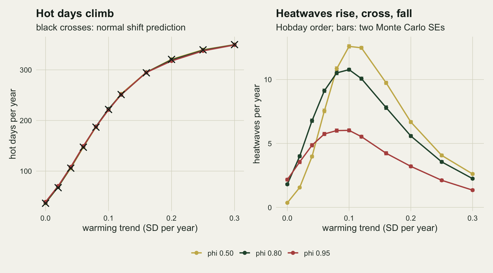
The rule order stays in play under warming. At phi 0.8 the merge-first count is 3.18 with no trend, 1.8 times the Hobday count, while at 0.30 it is 1.76 against 2.25 for the Hobday order, because filling gaps merges the long events of a warm decade still further. For phi 0.5 the gap is wider still at low trends: 5.96 against 1.55 at 0.02. A trend estimated from counts made with one implementation and compared with counts made with the other would be comparing different estimators.
The crossing needs no warming
The main thing the warming arm changes is the share of days above the threshold, and the hot-days check above shows that share follows a normal shift. So the stationary records can be asked the same question directly. The chunk below takes new stationary records of 100 decades for each persistence level, with no trend and no seasonal cycle, and lowers the true threshold so that 5, 10, … 95 per cent of days are hot. It also scores each record at exactly the share of hot days measured at each point of the warming grid.
For comparison it prints a closed form. If the hot-day indicator were a two-state Markov chain, with p_ch the probability of a cool day followed by a hot one, a the probability that a hot day is followed by another and b the same for cool days, the runs of at least five hot days would start at 365 p_ch a^4 per year, and the Hobday count would be that times one minus the chance that the run before lies within two cool days and is itself kept, (1 - b^2) a^4. For the AR(1) anomaly p_ch is a bivariate normal probability, computed below by one numerical integral.
share_grid <- seq(0.05, 0.95, by = 0.05)
n_dec_sw   <- 100

# two-state Markov approximation of the Hobday count per year
markov_hw <- function(phi, p_hot, min_len = min_len_hw, max_gap = max_gap_hw) {
  u_thr <- qnorm(1 - p_hot)
  up_dens <- function(z) {
    pnorm((u_thr - phi * z) / sqrt(1 - phi^2), lower.tail = FALSE) * dnorm(z)
  }
  p_ch <- integrate(up_dens, -Inf, u_thr)$value   # P(cool today, hot tomorrow)
  a_hh <- 1 - p_ch / p_hot                         # P(hot | hot)
  b_cc <- 1 - p_ch / (1 - p_hot)                   # P(cool | cool)
  runs <- 365 * p_ch * a_hh^(min_len - 1)
  runs * (1 - (1 - b_cc^max_gap) * a_hh^(min_len - 1))
}

set.seed(20164)
yr_in_dec <- rep(rep(0:9, each = n_doy), n_dec_sw)  # year within each decade
sweep_parts <- lapply(phi_warm, function(phi) {
  x_sw  <- ar1_series(n_dec_sw * dec_len, phi)
  w_sub <- warm_tab[warm_tab$phi == phi, ]
  curve_part <- do.call(rbind, lapply(share_grid, function(p_hot) {
    counts <- per_decade(hobday_events(x_sw > qnorm(1 - p_hot)), n_dec_sw) / 10
    data.frame(phi = phi, share = p_hot, events = mean(counts),
               se = sd(counts) / sqrt(n_dec_sw), markov = markov_hw(phi, p_hot))
  }))
  matched_part <- data.frame(phi = phi, trend = w_sub$trend,
    share = w_sub$days / 365, warm = w_sub$events,
    stat = vapply(w_sub$days / 365, function(p_hot)
      hobday_events(x_sw > qnorm(1 - p_hot))$n / (n_dec_sw * 10), numeric(1)),
    # same records with the trend climbing inside each decade, exact constant
    # threshold set so the decade has the same average share of hot days
    climb = vapply(seq_len(nrow(w_sub)), function(i) {
      q_cl <- uniroot(function(q) mean(pnorm(w_sub$trend[i] * (0:9) - q)) -
                        w_sub$days[i] / 365, c(-10, 10))$root
      hobday_events(x_sw + w_sub$trend[i] * yr_in_dec > q_cl)$n / (n_dec_sw * 10)
    }, numeric(1)))
  list(curve = curve_part, matched = matched_part)
})
sweep_tab   <- do.call(rbind, lapply(sweep_parts, `[[`, "curve"))
matched_tab <- do.call(rbind, lapply(sweep_parts, `[[`, "matched"))
matched_tab$gap <- matched_tab$warm - matched_tab$stat

sw <- function(phi, p_hot, col) {
  sweep_tab[[col]][sweep_tab$phi == phi & abs(sweep_tab$share - p_hot) < 1e-9]
}
diff_lo_hi <- sweep_tab$events[sweep_tab$phi == 0.5] - sweep_tab$events[sweep_tab$phi == 0.95]
i_cross    <- which(diff_lo_hi > 0)[1]
cross_share <- share_grid[i_cross - 1] + 0.05 * (-diff_lo_hi[i_cross - 1]) /
  (diff_lo_hi[i_cross] - diff_lo_hi[i_cross - 1])
sw05 <- sweep_tab[sweep_tab$phi == 0.5, ]
sw95 <- sweep_tab[sweep_tab$phi == 0.95, ]
markov_gap05 <- max(abs(sw05$events - sw05$markov))
markov_gap95 <- max(abs(sw95$events - sw95$markov))
peak05_share <- sw05$share[which.max(sw05$events)]
max_se_sw    <- max(sweep_tab$se)
early   <- matched_tab$trend <= 0.06
gap_early <- max(abs(matched_tab$gap[early]))
late_min  <- matched_tab[which.min(matched_tab$gap), ]
late_gap  <- matched_tab$gap[!early]
late_max  <- matched_tab[!early, ][which.max(late_gap), ]
markov_peak05 <- sw05$share[which.max(sw05$markov)]
climb_resid <- max(abs(matched_tab$warm - matched_tab$climb))
mt <- function(phi, tr, col) matched_tab[[col]][matched_tab$phi == phi & abs(matched_tab$trend - tr) < 1e-9]
In the stationary records the phi 0.5 count overtakes the phi 0.95 count once 34 per cent of days are hot (interpolated between grid points; the largest Monte Carlo SE on this grid is 0.08). At 30 per cent the counts are 4.01 and 5.01, at 40 per cent 7.28 and 5.89. Nothing in these records warms. The same crossing therefore appears under any rule that lets through more than that share of days, such as a 60th percentile threshold, or a threshold carried over from a much colder site.
Scored at the share of hot days measured at a trend of 0.06, the stationary records give 7.45 at phi 0.5 and 5.94 at phi 0.95, against 7.55 and 5.74 in the warming records. Up to that trend no warming count differs from its matched stationary count by more than 0.24. Further right the warming count is lower in 20 of the 21 grid points, by up to 2.35 at phi 0.50 and a trend of 0.16; the largest difference the other way is 0.46, at phi 0.50 and a trend of 0.30. Inside the counted decade the share of hot days is not constant: it climbs from year to year, and averaging a curve that bends downwards over a spread of shares gives less than its value at the average share. The chunk tests this by adding the same within-decade climb to the stationary records, with an exact constant threshold and no seasonal cycle. That gives 9.71 at phi 0.50 and a trend of 0.16, against 9.74 in the warming records, and across the whole grid the two never differ by more than 0.17; the climb inside the decade, not the estimated seasonal threshold, accounts for the shortfall. Warming against a fixed baseline moves each site along the stationary curve, averaged over the shares its counted decade passes through, and the curve is where the peak and the crossing live.
The closed form carries most of the low-persistence curve. At phi 0.5 it differs from the simulated count by at most 0.43 heatwaves per year across the whole grid, it puts the peak at the same share of hot days as the simulation, 70 per cent (the raw rate of cool-to-hot transitions peaks at half the days by symmetry, and the run-length terms move the peak to higher shares), and it falls towards zero as every day becomes hot. At phi 0.95 it fails: at half the days hot it gives 10.54 against a simulated 6.34, and the largest gap on the grid is 4.30. A thresholded AR(1) series is not a Markov chain: after a long hot run the anomaly tends to sit further above the threshold than after a single hot day, so it is more likely to stay hot, and the stronger the persistence the more that memory matters. For persistent anomalies the count cannot be written down from the share of hot days and one transition probability; it has to be simulated, or counted.
ggplot(sweep_tab, aes(share, events, colour = factor(sprintf("phi %.2f", phi)))) +
  geom_line(aes(y = markov), linetype = "dashed", linewidth = 0.6) +
  geom_line(linewidth = 0.9) +
  geom_point(data = matched_tab, aes(share, warm), shape = 1, size = 2.6,
             stroke = 0.9) +
  scale_colour_manual(values = c(te_gold, te_forest, te_rust), name = NULL) +
  scale_x_continuous(labels = function(v) sprintf("%.0f%%", 100 * v)) +
  labs(x = "share of days above the threshold", y = "heatwaves per year",
       title = "The count follows the share of hot days",
       subtitle = "solid: stationary records; dashed: Markov closed form; circles: warming grid") +
  theme_datasheet() +
  theme(legend.position = "bottom")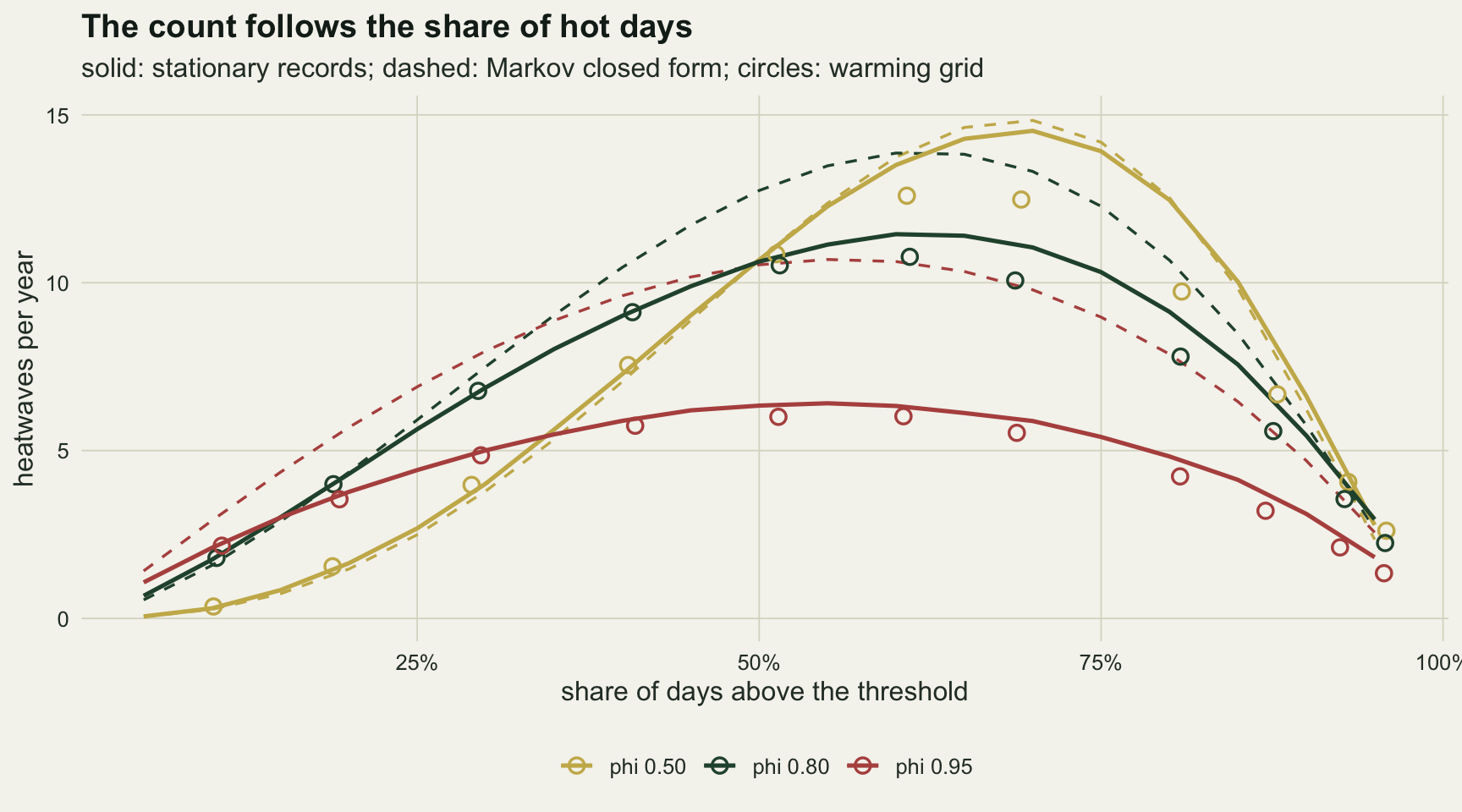
Days, duration and intensity do not turn round
The count falls because events merge, so metrics that add up the heat inside events rather than counting the events keep rising. Heatwave days (days inside an event) and cumulative intensity (the sum over those days of the temperature above the climatological mean, in anomaly units) are two of them. Perkins and Alexander (2013) proposed measuring terrestrial heatwaves on several aspects at once (the number of events, their length, the number of days taking part, and their magnitude) for this reason: each answers a different question about the same hot days.
ev_days_mono <- all(vapply(phi_warm, function(phi)
  all(diff(warm_tab$ev_days[warm_tab$phi == phi]) > 0), logical(1)))
cum_mono <- all(vapply(phi_warm, function(phi)
  all(diff(warm_tab$cum_int[warm_tab$phi == phi]) > 0), logical(1)))
Across all three persistence levels, heatwave days rise at every step of the trend grid, and cumulative intensity does too. At phi 0.8 heatwave days go from 13.1 to 188.4 per year at the trend where the count peaks and on to 347.9, while the pooled mean event duration (heatwave days divided by heatwaves) goes from 7.2 days to 17.5 and then 154.9. Past the peak the count falls because the events it counts grow long enough to swallow one another.
p_dur <- ggplot(warm_plot, aes(trend, dur, colour = persistence)) +
  geom_line(linewidth = 0.8) +
  geom_point(size = 1.8) +
  scale_y_log10() +
  scale_colour_manual(values = c(te_gold, te_forest, te_rust), name = NULL) +
  labs(x = "warming trend (SD per year)", y = "pooled mean duration (days, log scale)",
       title = "Events lengthen") +
  theme_datasheet()

p_cum <- ggplot(warm_plot, aes(trend, cum_int, colour = persistence)) +
  geom_line(linewidth = 0.8) +
  geom_point(size = 1.8) +
  scale_colour_manual(values = c(te_gold, te_forest, te_rust), name = NULL) +
  labs(x = "warming trend (SD per year)",
       y = "cumulative intensity per year (SD days)",
       title = "Heat in events keeps rising") +
  theme_datasheet()

(p_dur | p_cum) +
  plot_layout(guides = "collect") +
  plot_annotation(theme = theme_datasheet()) &
  theme(legend.position = "bottom")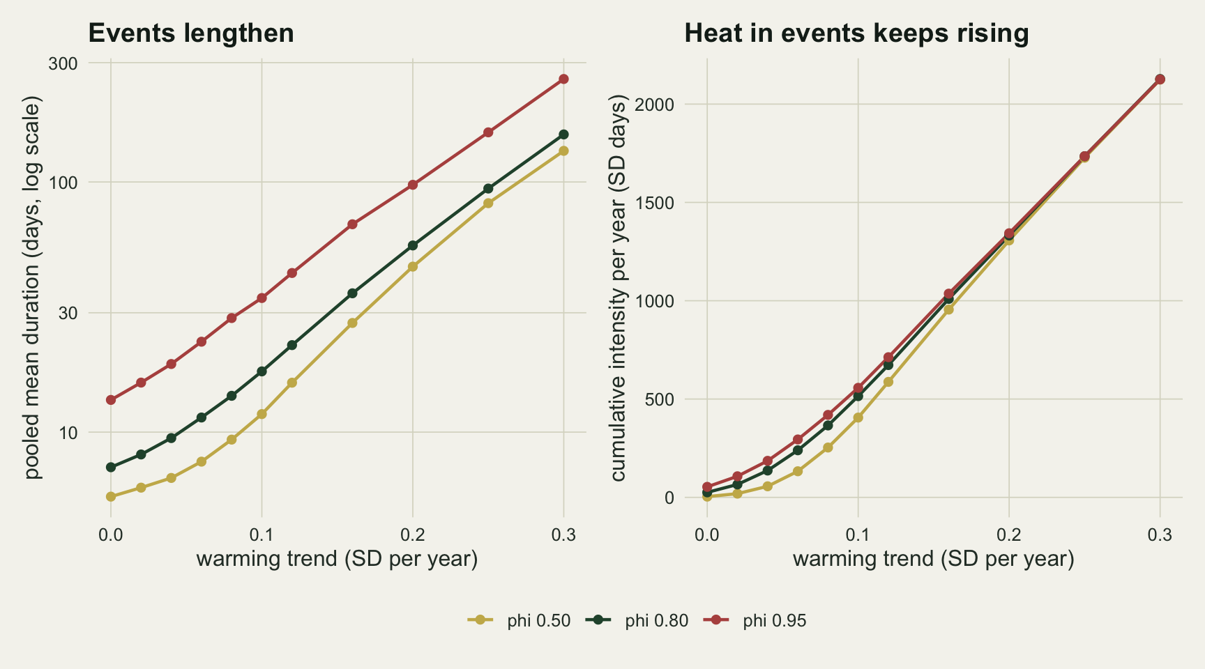
The baseline, briefly
The same records at phi 0.8 were also scored against two other baselines: a recent ten-year baseline (years 21 to 30), and a shifting baseline in which the linear trend fitted to the 40 annual means is removed before the threshold is computed, the shifting baseline Jacox (2019) discussed. Schlegel and colleagues (2019) ran their own sensitivity tests on detrended anomalies, compared 10-year with 30-year records, and found that an added linear trend changed the count and duration of detected events more than shortening the record did.
With no trend the three baselines give 1.80, 2.00 and 1.79 heatwaves per year (fixed, recent ten years, shifting), and 37.7, 40.2 and 37.2 hot days; the ten-year baseline estimates the percentile from a third of the data and lets more days through. At a trend of 0.04 the counts are 6.78, 4.46 and 1.79, at 0.12 they are 10.07, 9.27 and 1.88, and at 0.30 they are 2.25, 5.70 and 1.81. The recent baseline sits closer in time to the counted decade and lets fewer days through (166.0 against 250.8 hot days at 0.12). Whether that lowers or raises the count depends on which side of the peak of the count curve the site sits: from a trend of 0.02 to 0.12 the recent baseline gives fewer heatwaves than the fixed one, and from 0.16 on, where the fixed-baseline count is already falling, it gives more. The shifting baseline removes the warming by construction and returns the stationary count; it answers a different question (is variability around the trend more extreme?) rather than giving a better answer to the same one. Drought indices for ecologists covers the same choice for a standardised index.
What to report
Name the rule order, not only the numbers in the rule. “At least five days, gaps of two days or less joined” is compatible with counts that differed by a factor of 6.7 on the same stationary data at phi 0.5 and 1.8 at phi 0.8. Quoting Hobday and colleagues’ gap sentence (gaps of two days or less are joined only between events of five days or more), or citing an implementation that follows it such as heatwaveR, closes the room for the merge-first misreading.
Report the lag-one autocorrelation of the daily anomalies with any heatwave count, and compare counts between sites only when their persistence is similar. The stationary count at an unchanged ten per cent of hot days moved by a factor of 7.1 between phi 0.5 and 0.9 under the Hobday order, and the ranking of sites by count depends on the share of days above the threshold, so it reverses under warming and between threshold choices.
Report heatwave days or cumulative intensity next to the count, and treat the count as a partition of those days rather than as a heat index. For organisms the relevant quantity is usually the dose (days above a tolerance, or accumulated excess heat), and the count is the one metric in the set that can fall while the dose rises. A decline in heatwave frequency at a warming site is a prompt to look at duration before it is a finding.
State the baseline period and whether it is fixed or shifting. With a fixed baseline, a count trend mixes the change in mean with any change in variability; with a shifting baseline, the mean change is removed on purpose.
Honest limits
The anomaly is a first-order autoregressive process with normal innovations and constant variance. Real temperature anomalies have longer memory, skewed tails and seasonally varying variance and persistence, and sea surface temperatures in particular are more persistent than air temperatures. At ten per cent of hot days the direction of the persistence and rule-order effects should carry over; at high shares of hot days both reverse, as the warming section shows. Their size is specific to this process, and phi was not estimated from any real logger.
The warming is a straight line in the mean. A change in variance with no change in mean alters counts without altering the mean, and a step change or an accelerating trend moves the peak of the count curve. The trend grid is in anomaly standard deviations per year, so its right half corresponds to very fast warming for most places; it is there to show the shape of the curve, not a forecast.
Events are counted inside a ten-year window. An event running across the start or end of the window is cut, and in the stationary section an event is assigned to the decade in which it starts. At the largest trends, where a single event can last months, the window edge shortens the mean duration shown and the counts there should be read as approximate.
The threshold follows the heatwaveR defaults, but only the basic Hobday metrics were computed. The categories of Hobday and colleagues’ later scheme, the second threshold and minimum duration that heatwaveR allows, and cold spells were not simulated. The seasonal cycle is a single sine wave with a fixed amplitude; a sharper seasonal cycle widens the pooled window and makes the threshold noisier near the solstices.
Merge-first is a misreading of the definition, not a published alternative, and no study is known here to have used it. Whether one did cannot be read from the counts alone, which is the practical reason for quoting the gap rule in full. The Markov closed form is an approximation checked against the simulation on this grid only; it is not derived for seasonal or trending records.
References
Hobday AJ, Alexander LV, Perkins SE, Smale DA, Straub SC, Oliver ECJ, Benthuysen JA, Burrows MT, Donat MG, Feng M, Holbrook NJ, Moore PJ, Scannell HA, Sen Gupta A, Wernberg T 2016 Progress in Oceanography 141:227-238 (10.1016/j.pocean.2015.12.014)
Schlegel RW, Smit AJ 2018 Journal of Open Source Software 3(27):821 (10.21105/joss.00821)
Jacox MG 2019 Nature 571(7766):485-487 (10.1038/d41586-019-02196-1)
Schlegel RW, Oliver ECJ, Hobday AJ, Smit AJ 2019 Frontiers in Marine Science 6:737 (10.3389/fmars.2019.00737)
Perkins SE, Alexander LV 2013 Journal of Climate 26(13):4500-4517 (10.1175/JCLI-D-12-00383.1)