---
title: "Checking a multi-model analysis"
description: "Three diagnostics for a multi-model analysis in R: selection bias and the winner's curse, candidate-set dependence, and when the truth is not in the set."
date: "2026-06-24 09:00"
date-modified: "2026-10-14"
categories: [R, multimodel inference, model averaging, model checking, ggplot2, ecology tutorial]
image: thumbnail.png
image-alt: "Residuals from a best main-effects model plotted against an omitted interaction term, showing clear leftover structure."
---
*Corrected 14 October 2026: the post said that adding a redundant variable moved the ranking and could rewrite the importance rankings or make a strong effect look weak; it now says the weights and the importance moved, that the duplicate dilutes the support for the variable it copies and that a strong effect can be made to look weaker, since in the example the best model and the order of the original predictors did not change.*
*Corrected 1 October 2026: the post said that any coefficient that helped a model win is, on average, larger in the winning model than its true value; it now limits that to coefficients that win only narrowly, and says that a strong effect selected in almost every data set is barely affected.*
A multi-model analysis produces confident-looking output: a ranked table, Akaike weights, a summed weight for each predictor, maybe a model-averaged prediction. None of that output tells you whether the exercise was sound. The weights are internally consistent by construction; they describe support relative to the candidate set, and they stay tidy even when the set is the wrong set or the fitting has quietly overfitted.
This post gives three checks that catch the common failures. The first asks whether selection has inflated the effects it chose. The second asks whether the weights would survive a change to the candidate set. The third asks whether the truth is even reachable from the models on offer. Each is a short simulation in base R, and each corresponds to a way that a clean-looking model table can mislead.
These build on [Akaike weights](../akaike-weights/) and the [coefficient cautions](../model-averaged-coefficients/); here the focus is on what to check before trusting any of it.
## Diagnostic one: selection bias and the winner's curse
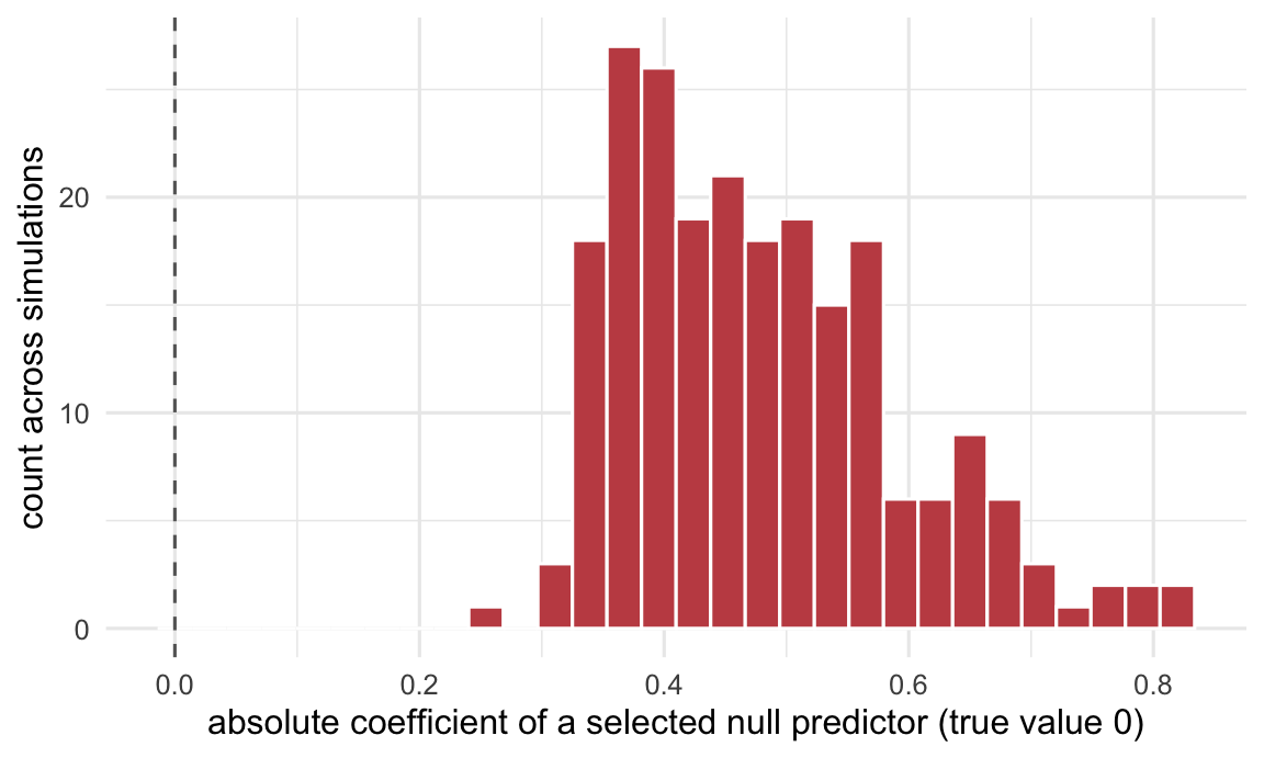
When you search a set of models and keep the best, the winner is best partly because it captured real signal and partly because it caught favourable noise. A coefficient that only narrowly helped a model win is, on average, larger in that winning model than its true value; a strong effect that is selected in almost every data set is barely affected, because selection discards almost none of its estimates. For a predictor with no real effect that nonetheless gets selected, this is the winner's curse: it appears only when its sampling noise happened to be large, so its estimated effect is systematically inflated.
The simulation gives six candidate predictors to a response driven by only the first. Every subset is fitted, the best by AICc is kept, and we track how often a truly null predictor sneaks into the winner and how large its coefficient looks when it does.
```{r selbias}
aicc <- function(m) { k <- length(coef(m)) + 1; N <- nobs(m); AIC(m) + 2 * k * (k + 1) / (N - k - 1) }
P <- 6; n <- 70
preds   <- paste0("x", 1:P)
subsets <- unlist(lapply(0:P, function(k) combn(preds, k, simplify = FALSE)), recursive = FALSE)
forms   <- vapply(subsets, function(s)
  if (length(s) == 0) "y ~ 1" else paste("y ~", paste(s, collapse = " + ")), character(1))

# one large fixed hold-out set representing the truth (only x1 has an effect)
set.seed(6061)
Nte <- 3000
Xte <- as.data.frame(matrix(rnorm(Nte * P), Nte, P)); names(Xte) <- preds
Xte$y <- 2 + 1.0 * Xte$x1 + rnorm(Nte, 0, 2.0)
r2 <- function(m, D) { yh <- predict(m, D); 1 - sum((D$y - yh)^2) / sum((D$y - mean(D$y))^2) }

set.seed(606)
reps <- 300
retained <- 0; null_coefs <- c(); r2_in <- c(); r2_out <- c()
for (i in seq_len(reps)) {
  X <- as.data.frame(matrix(rnorm(n * P), n, P)); names(X) <- preds
  X$y <- 2 + 1.0 * X$x1 + rnorm(n, 0, 2.0)
  fits <- lapply(forms, function(f) lm(as.formula(f), data = X))
  best <- fits[[which.min(vapply(fits, aicc, numeric(1)))]]
  chosen <- names(coef(best))[-1]
  nulls  <- setdiff(preds, "x1")                 # x2..x6 have no true effect
  got    <- intersect(chosen, nulls)
  retained <- retained + (length(got) > 0)
  for (v in got) null_coefs <- c(null_coefs, abs(coef(best)[v]))
  r2_in  <- c(r2_in,  r2(best, X))
  r2_out <- c(r2_out, r2(best, Xte))
}
c(p_null_retained = retained / reps,
  mean_null_coef  = mean(null_coefs),
  r2_in  = mean(r2_in),
  r2_out = mean(r2_out))
```
```{r selnums}
p_ret   <- retained / reps
mean_nc <- mean(null_coefs)
r2i     <- mean(r2_in); r2o <- mean(r2_out)
```
A truly null predictor lands in the best model in `r sprintf("%.0f", p_ret * 100)` per cent of datasets, and when one does, its estimated coefficient averages `r sprintf("%.2f", mean_nc)` in absolute value, despite a true effect of exactly zero. That is the winner's curse made numeric: selection only keeps null predictors whose noise was large, so the kept ones look substantial. The in-sample fit tells the same story from the other side: the best model explains `r sprintf("%.1f", r2i * 100)` per cent of the variance in its own data but only `r sprintf("%.1f", r2o * 100)` per cent on fresh data from the same process, an optimism gap of `r sprintf("%.1f", (r2i - r2o) * 100)` percentage points that comes entirely from fitting to noise the model then cannot reproduce.
```{r fig-nullcoef}
#| fig-cap: "Absolute coefficients of truly null predictors on the occasions they were selected into the best model. The true value is zero (dashed), yet the selected estimates cluster well away from it: the winner's curse."
#| fig-alt: "Histogram of absolute coefficient values for null predictors that were selected, piling up around one-third to one-half rather than at the dashed zero line."
#| fig-width: 6
#| fig-height: 3.6
library(ggplot2)
te_canvas <- theme(plot.background  = element_rect(fill = "#f5f4ee", colour = NA),
                   panel.background = element_rect(fill = "#f5f4ee", colour = NA))
ggplot(data.frame(coef = null_coefs), aes(coef)) +
  geom_histogram(bins = 30, fill = "#c44e52", colour = "white") +
  geom_vline(xintercept = 0, linetype = "dashed", colour = "grey40") +
  labs(x = "absolute coefficient of a selected null predictor (true value 0)",
       y = "count across simulations") +
  theme_minimal(base_size = 12) + te_canvas
```
The practical check on your own analysis: compare the fit of your selected or averaged model on held-out data against its in-sample fit. A large drop is the optimism this simulation manufactures on purpose. The remedy is to keep candidate sets small and grounded in prior hypotheses rather than throwing in every measured variable, a point Anderson and Burnham make repeatedly, and to distrust any effect that appears only after a search over many models.
## Diagnostic two: candidate-set dependence
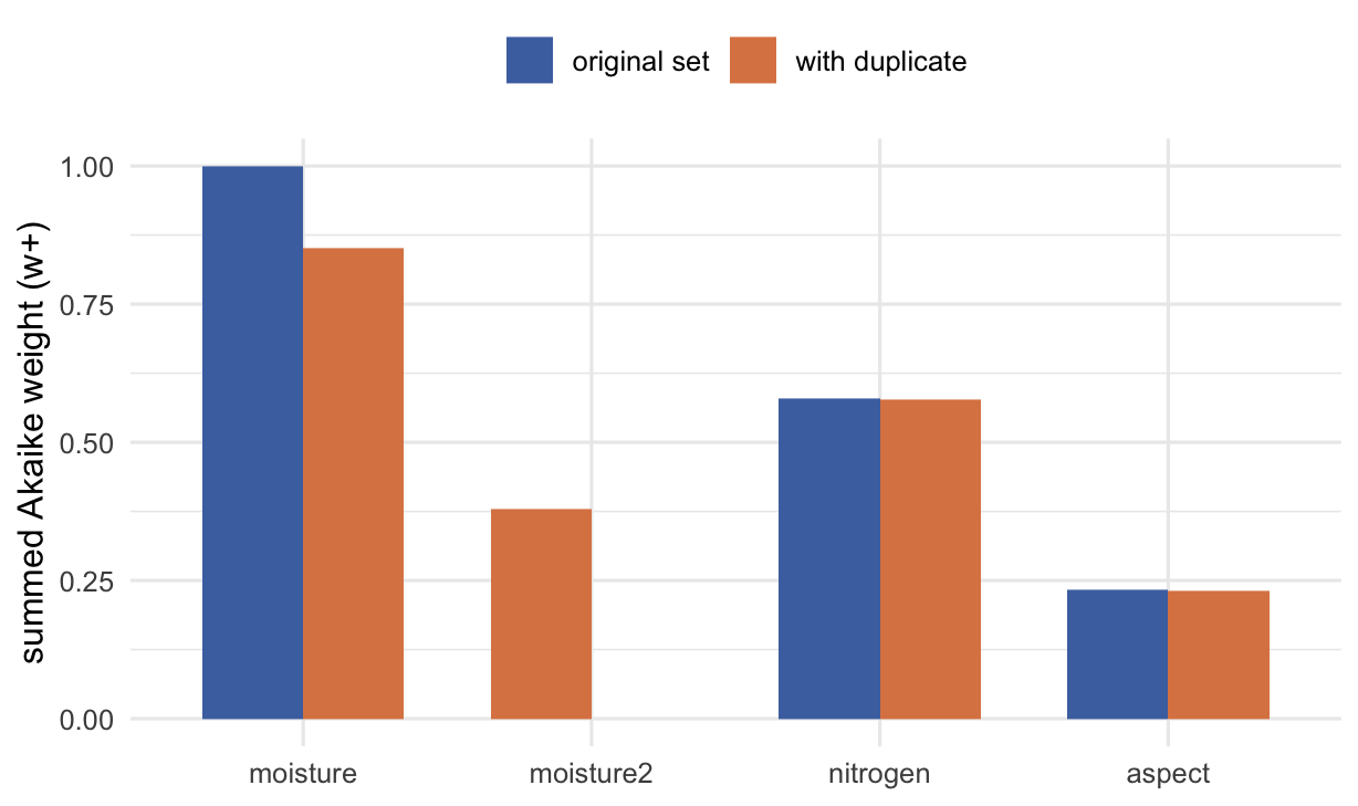
Akaike weights are computed relative to the set. Change the set and the weights change, sometimes drastically, even when the data are identical. The most common way this bites is a redundant predictor: two variables that measure nearly the same thing split the weight and the summed importance between them, so a strong effect can be made to look weaker just by adding its near-copy to the candidates.
We take the grassland example, add a second moisture-like variable correlated at 0.97 with the first, and compare the weights before and after.
```{r setdep}
set.seed(202)
n2 <- 55
moisture <- rnorm(n2); nitrogen <- rnorm(n2); aspect <- rnorm(n2)
biomass  <- 2 + 1.0 * moisture + 0.22 * nitrogen + 0 * aspect + rnorm(n2, 0, 1.6)
set.seed(2021)
moisture2 <- moisture + rnorm(n2, 0, 0.25)     # a near-duplicate sensor
cor_dup <- cor(moisture, moisture2)

weights_for <- function(vars, data) {
  ss <- unlist(lapply(0:length(vars), function(k) combn(vars, k, simplify = FALSE)), recursive = FALSE)
  ff <- vapply(ss, function(s)
    if (length(s) == 0) "biomass ~ 1" else paste("biomass ~", paste(s, collapse = " + ")), character(1))
  fits <- lapply(ff, function(f) lm(as.formula(f), data = data))
  w <- exp(-0.5 * (vapply(fits, aicc, numeric(1)) - min(vapply(fits, aicc, numeric(1))))); w <- w / sum(w)
  imp <- vapply(vars, function(v) sum(w[vapply(ss, function(s) v %in% s, logical(1))]), numeric(1))
  list(best_weight = max(w), importance = imp)
}

dat <- data.frame(biomass, moisture, nitrogen, aspect, moisture2)
before <- weights_for(c("moisture", "nitrogen", "aspect"), dat)
after  <- weights_for(c("moisture", "nitrogen", "aspect", "moisture2"), dat)
```
```{r setdepnums}
bw_before <- before$best_weight; bw_after <- after$best_weight
imp_moist_before <- before$importance["moisture"]
imp_moist_after  <- after$importance["moisture"]
imp_moist2_after <- after$importance["moisture2"]
```
The added sensor correlates with the original at `r sprintf("%.2f", cor_dup)`, so it carries essentially the same information. Before adding it, the top model holds a weight of `r sprintf("%.3f", bw_before)` and moisture has summed weight `r sprintf("%.2f", imp_moist_before)`. After adding it, the top model's weight falls to `r sprintf("%.3f", bw_after)`, because the duplicate spawns a family of near-equivalent models that share the support, so no single model dominates any more. Moisture's summed weight leaks from `r sprintf("%.2f", imp_moist_before)` to `r sprintf("%.2f", imp_moist_after)` with the duplicate collecting `r sprintf("%.2f", imp_moist2_after)`. The weights and the importance both moved, purely from adding a redundant variable, while the underlying effect is exactly as strong as before.
```{r fig-setdep}
#| fig-cap: "Summed weights before and after adding a near-duplicate moisture sensor. The strong moisture effect is split across two proxies, so both look weaker, while the true signal is unchanged."
#| fig-alt: "Grouped bar chart of summed weights for each predictor, before and after adding a duplicate. Moisture's bar drops and the new duplicate takes a share, splitting the importance."
#| fig-width: 6.4
#| fig-height: 3.8
impdf <- rbind(
  data.frame(predictor = names(before$importance), wplus = as.numeric(before$importance), set = "original set"),
  data.frame(predictor = names(after$importance),  wplus = as.numeric(after$importance),  set = "with duplicate"))
impdf$predictor <- factor(impdf$predictor, levels = c("moisture", "moisture2", "nitrogen", "aspect"))
ggplot(impdf, aes(predictor, wplus, fill = set)) +
  geom_col(position = position_dodge(preserve = "single"), width = 0.7) +
  scale_fill_manual(values = c("original set" = "#4c72b0", "with duplicate" = "#dd8452"), name = NULL) +
  labs(x = NULL, y = "summed Akaike weight (w+)") +
  theme_minimal(base_size = 12) + te_canvas + theme(legend.position = "top")
```
The check: before reading importance off summed weights, ask whether any candidates are near-duplicates or strongly collinear. If they are, the weights are describing your variable list as much as your ecology. Prune redundant predictors, or treat correlated variables as a group rather than competitors.
## Diagnostic three: when the truth is not in the set
The Akaike weight of the best model says it is the best of the candidates. It says nothing about whether the candidates are any good. If the process generating the data has structure that none of your models can represent, one model will still win, often with a comfortable weight, and the analysis will look settled while missing the mechanism entirely.
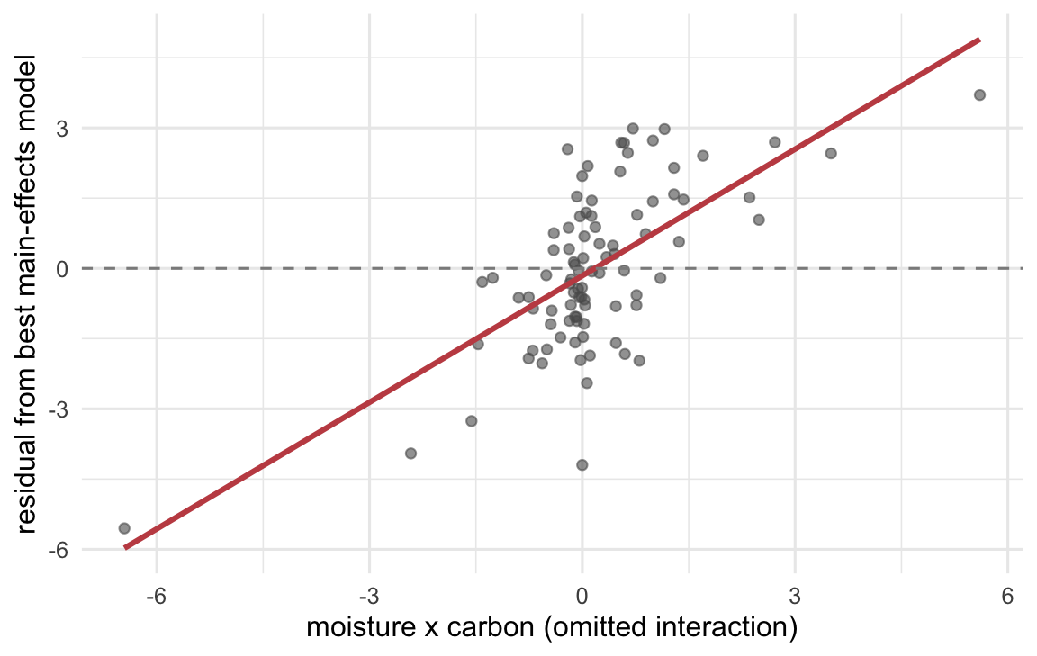
Here the truth includes an interaction between moisture and carbon, but the candidate set contains main effects only. We fit the main-effects models, note the weight on the winner, then check it against a large hold-out and against an oracle model that does include the interaction.
```{r truthset}
set.seed(808)
n3 <- 90
moisture <- rnorm(n3); carbon <- rnorm(n3); aspect <- rnorm(n3)
biomass  <- 2 + 1.0 * moisture + 0.8 * carbon + 1.3 * moisture * carbon + 0 * aspect + rnorm(n3, 0, 1.5)
dt <- data.frame(biomass, moisture, carbon, aspect)

main_vars <- c("moisture", "carbon", "aspect")
ss <- unlist(lapply(0:3, function(k) combn(main_vars, k, simplify = FALSE)), recursive = FALSE)
ff <- vapply(ss, function(s)
  if (length(s) == 0) "biomass ~ 1" else paste("biomass ~", paste(s, collapse = " + ")), character(1))
fits <- lapply(ff, function(f) lm(as.formula(f), data = dt))
w <- exp(-0.5 * (vapply(fits, aicc, numeric(1)) - min(vapply(fits, aicc, numeric(1))))); w <- w / sum(w)
best_i <- which.max(w)
best_main <- fits[[best_i]]
best_weight <- w[best_i]
```
```{r truthnums}
set.seed(8081)
Dte <- data.frame(moisture = rnorm(4000), carbon = rnorm(4000), aspect = rnorm(4000))
Dte$biomass <- 2 + 1.0 * Dte$moisture + 0.8 * Dte$carbon + 1.3 * Dte$moisture * Dte$carbon + rnorm(4000, 0, 1.5)
r2 <- function(m, D) { yh <- predict(m, D); 1 - sum((D$biomass - yh)^2) / sum((D$biomass - mean(D$biomass))^2) }
oracle <- lm(biomass ~ moisture * carbon, data = dt)
r2_best   <- r2(best_main, Dte)
r2_oracle <- r2(oracle, Dte)
p_interaction <- summary(lm(resid(best_main) ~ I(moisture * carbon), data = dt))$coefficients["I(moisture * carbon)", "Pr(>|t|)"]
```
```{r sci-tex-helper}
#| include: false
sci_tex <- function(x, digits = 2) {
s <- formatC(x, format = "e", digits = digits)
paste0("$", sub("e.*", "", s), " \\times 10^{", as.integer(sub(".*e", "", s)), "}$")
}
```
The best main-effects model, `r sub("biomass ~ ", "", ff[best_i])`, carries an Akaike weight of `r sprintf("%.2f", best_weight)`, which on its own would read as solid support. Yet on fresh data it explains only `r sprintf("%.1f", r2_best * 100)` per cent of the variance, while the oracle model with the interaction reaches `r sprintf("%.1f", r2_oracle * 100)` per cent. The gap is the signal the candidate set could not represent, and the weight had no way to reveal it, because the weight only compares models that were offered.
The diagnostic that does reveal it is the residual plot. Regress the best model's residuals on the omitted interaction term, and the leftover structure is unmistakable.
```{r fig-resid}
#| fig-cap: "Residuals of the best main-effects model against the omitted moisture-by-carbon product. The strong trend is the interaction the candidate set could not fit; the association is far beyond chance."
#| fig-alt: "Scatter plot of best-model residuals against the moisture-times-carbon product, with a clear rising trend line, showing systematic leftover structure."
#| fig-width: 6
#| fig-height: 3.8
rdf <- data.frame(product = dt$moisture * dt$carbon, resid = resid(best_main))
ggplot(rdf, aes(product, resid)) +
  geom_point(alpha = 0.6, colour = "grey35") +
  geom_smooth(method = "lm", se = FALSE, colour = "#c44e52", formula = y ~ x) +
  geom_hline(yintercept = 0, linetype = "dashed", colour = "grey55") +
  labs(x = "moisture x carbon (omitted interaction)", y = "residual from best main-effects model") +
  theme_minimal(base_size = 12) + te_canvas
```
The slope is significant at p = `r sci_tex(p_interaction, 1)`, a decisive signal that the residuals still contain structure keyed to a term the models never included. A high Akaike weight paired with residuals like these is the signature of a candidate set that is too small: the winner is the best of a bad lot. The fix is not more weighting but a better set, informed by plausible mechanisms, including the interactions and non-linearities the ecology suggests.
## Putting the three together
None of these failures shows up in the weights themselves, which is exactly why they are worth checking for. Selection bias inflates the effects a search happens to keep; candidate-set dependence lets a redundant variable dilute the support for the variable it copies; and a set that cannot represent the truth still crowns a confident winner. The three checks are cheap: a held-out fit for optimism, a look at collinearity and duplication before reading importance, and a residual plot against plausible omitted terms. Run them before the model table earns your trust, not after it has shaped the conclusions.
## References
Anderson DR, Burnham KP (2002) Journal of Wildlife Management 66(3):912-918 (10.2307/3803155)
Forstmeier W, Schielzeth H (2011) Behavioral Ecology and Sociobiology 65(1):47-55 (10.1007/s00265-010-1038-5)
Cade BS (2015) Ecology 96(9):2370-2382 (10.1890/14-1639.1)
## Related tutorials
- [Akaike weights and evidence ratios](../akaike-weights/)
- [Model-averaged coefficients: a caution](../model-averaged-coefficients/)
- [Checking a nonlinear model](../checking-a-nonlinear-model/)
- [AIC with missing values: the silent row drop](../model-selection-with-missing-values/)