---
title: "AIC with missing values: the silent row drop"
description: "R fits every model to whatever rows are complete for it, so an AIC table over covariates with different missingness ranks the gaps, not the ecology. Shown in R."
date: "2026-08-06 09:00"
categories: [R, model selection, AIC, missing data, ecology tutorial]
image: thumbnail.png
image-alt: "Four labelled points joined by a line, showing delta AIC rising steadily with the number of plots each candidate model was actually fitted to."
---
Field data has holes. The soil chemistry came back for most plots but not all, the canopy measurement was skipped when the weather turned, one logger failed in July. You build a candidate model set out of the covariates you have, run `AIC`, and read off the winner.
R will do this without complaint, and the answer can be entirely an artefact of where the holes are. Each model is fitted to the rows that are complete for the variables in that model, so different candidates are fitted to different data sets. Their log-likelihoods are sums over different numbers of rows, which makes them incomparable, and the incomparability points in a fixed direction: the model with the most missing data gets the best score.
## A candidate set where the answer is known
Two hundred plots. The response depends on `x1` and nothing else. `x2` is a covariate with no effect at all that is missing for thirty per cent of plots; `x3` is another null covariate missing for ten per cent.
```{r setup}
#| message: false
#| warning: false
library(ggplot2)

te_paper  <- "#f5f4ee"
te_ink    <- "#16241d"
te_body   <- "#2c3a31"
te_forest <- "#275139"
te_rust   <- "#b5534e"
te_gold   <- "#c9b458"
te_line   <- "#dad9ca"

theme_datasheet <- function() {
  theme_minimal(base_size = 12) +
    theme(plot.background  = element_rect(fill = te_paper, colour = NA),
          panel.background = element_rect(fill = te_paper, colour = NA),
          panel.grid.major = element_line(colour = te_line, linewidth = 0.3),
          panel.grid.minor = element_blank(),
          text             = element_text(colour = te_body),
          plot.title       = element_text(colour = te_ink, face = "bold"),
          axis.text        = element_text(colour = te_body))
}

make_plots <- function(n = 200, miss2 = 0.30, miss3 = 0.10) {
  d <- data.frame(x1 = rnorm(n), x2 = rnorm(n), x3 = rnorm(n))
  d$y <- 1.5 * d$x1 + rnorm(n)              # x2 and x3 do nothing
  d$x2[sample(n, round(miss2 * n))] <- NA
  d$x3[sample(n, round(miss3 * n))] <- NA
  d
}

set.seed(20260806)
plots <- make_plots()
colSums(is.na(plots))
```
The four candidates are the true model, the true model plus each null covariate, and the full model. Nothing here is subtle: `x2` and `x3` are noise, and any honest procedure should put `y ~ x1` first.
```{r candidates}
forms <- list(true      = y ~ x1,
              plus_x3   = y ~ x1 + x3,
              plus_x2   = y ~ x1 + x2,
              full      = y ~ x1 + x2 + x3)

fits <- lapply(forms, lm, data = plots)
aic_tab <- data.frame(model = names(forms),
                      rows  = sapply(fits, nobs),
                      aic   = sapply(fits, AIC))
aic_tab$delta <- aic_tab$aic - min(aic_tab$aic)
aic_tab[order(aic_tab$aic), ]
```
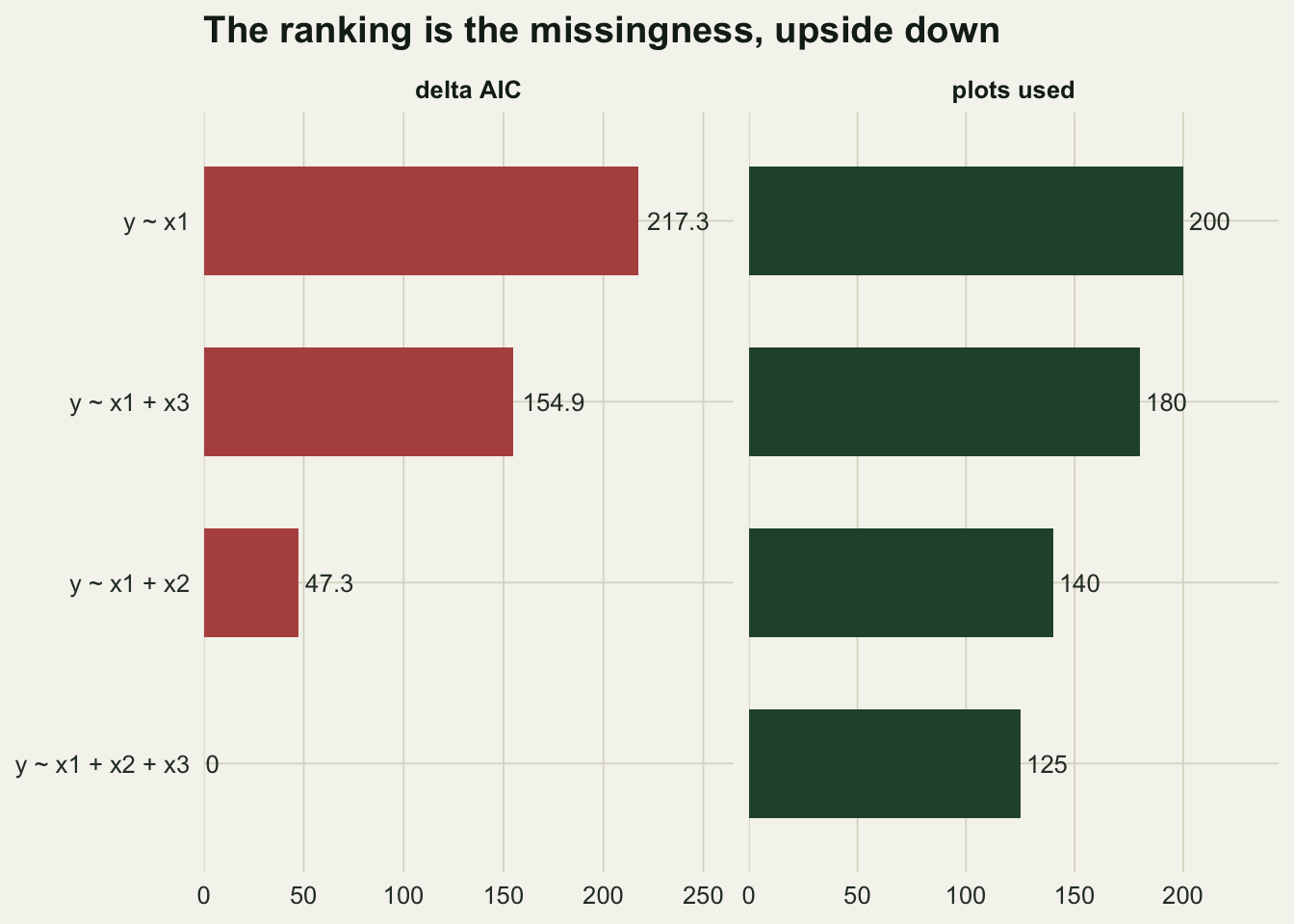
The full model wins, by `r sprintf("%.1f", aic_tab$delta[aic_tab$model == "true"])` AIC units over the model that generated the data. On the usual reading that is overwhelming support: a difference of ten is normally treated as decisive, and this is more than twenty times that.
Look at the `rows` column. The four models were fitted to `r aic_tab$rows[aic_tab$model == "true"]`, `r aic_tab$rows[aic_tab$model == "plus_x3"]`, `r aic_tab$rows[aic_tab$model == "plus_x2"]` and `r aic_tab$rows[aic_tab$model == "full"]` plots respectively. The AIC ordering is the row-count ordering read backwards. No warning was printed, and nothing in the printed table would tell a reader which models saw which plots unless they asked.
```{r fig-mirror}
#| fig-cap: "Delta AIC for the four candidates beside the number of plots each was actually fitted to."
#| fig-alt: "Two horizontal bar panels sharing the same four model labels. In the left panel the delta AIC bars grow as the row count in the right panel grows, so the best-scoring model is the one fitted to the fewest plots."
shown <- c(true = "y ~ x1", plus_x3 = "y ~ x1 + x3",
           plus_x2 = "y ~ x1 + x2", full = "y ~ x1 + x2 + x3")
mirror <- rbind(
  data.frame(model = aic_tab$model, panel = "delta AIC", value = aic_tab$delta),
  data.frame(model = aic_tab$model, panel = "plots used", value = aic_tab$rows))
mirror$model <- factor(shown[mirror$model],
                       levels = shown[aic_tab$model[order(aic_tab$rows)]])
mirror$panel <- factor(mirror$panel, levels = c("delta AIC", "plots used"))

ggplot(mirror, aes(y = model, x = value, fill = panel)) +
  geom_col(width = 0.6) +
  geom_text(aes(label = round(value, 1)), hjust = -0.15, size = 3.4,
            colour = te_body) +
  facet_wrap(~ panel, scales = "free_x") +
  scale_x_continuous(expand = expansion(mult = c(0, 0.22))) +
  scale_fill_manual(values = c("delta AIC" = te_rust, "plots used" = te_forest)) +
  labs(x = NULL, y = NULL, fill = NULL,
       title = "The ranking is the missingness, upside down") +
  theme_datasheet() +
  theme(legend.position = "none",
        strip.text = element_text(colour = te_ink, face = "bold"))
```
## Why the direction is fixed
The log-likelihood of a fitted model is a sum with one term per observation, and each term is negative for a continuous response with a density below one. Drop rows and you drop terms, so the log-likelihood rises towards zero and the AIC falls. The penalty for parameters is two per parameter, which is nowhere near enough to compensate for losing sixty rows.
The arithmetic is worth seeing once, because it makes clear that this is not a subtle statistical effect but a bookkeeping error.
```{r arithmetic}
per_row <- sapply(fits, function(m) as.numeric(logLik(m)) / nobs(m))
round(rbind(total_loglik = sapply(fits, function(m) as.numeric(logLik(m))),
            rows         = sapply(fits, nobs),
            per_row      = per_row), 3)
```
Per observation the four models fit almost identically, spanning `r sprintf("%.3f", diff(range(per_row)))` of a log-likelihood unit. It is only when each is multiplied by its own row count that they separate, and they separate in proportion to how much data each one threw away.
## Refit on the same plots and the ordering reverses
The repair is to decide the data set before the model set. Take the rows that are complete for every variable that appears anywhere in the candidate list, and fit all four to those.
```{r complete}
vars <- c("y", "x1", "x2", "x3")
common <- plots[complete.cases(plots[, vars]), ]

fits_c <- lapply(forms, lm, data = common)
tab_c  <- data.frame(model = names(forms),
                     rows  = sapply(fits_c, nobs),
                     aic   = sapply(fits_c, AIC))
tab_c$delta <- tab_c$aic - min(tab_c$aic)
tab_c[order(tab_c$aic), ]
```
All four are now fitted to the same `r tab_c$rows[1]` plots, and the true model is first with the two single-additions within `r sprintf("%.1f", max(tab_c$delta[tab_c$model %in% c("plus_x2", "plus_x3")]))` AIC units and the full model `r sprintf("%.1f", tab_c$delta[tab_c$model == "full"])` behind. That is the pattern AIC is supposed to produce for a null covariate: a penalty of about two per useless parameter, and no support for the elaboration.
The cost is visible too. The analysis now uses `r tab_c$rows[1]` of the original `r nrow(plots)` plots, because the union of the missingness patterns is larger than either alone. That is a real loss and it is the subject of a different decision, but it is a loss you can see and argue about, rather than one that quietly rewrites the ranking.
## How far the problem scales
The size of the artefact is a function of how much data the extra covariate is missing, and it is monotone.
```{r sweep}
sweep_miss <- function(fracs, reps = 40) {
  out <- data.frame()
  for (f in fracs) {
    gaps <- replicate(reps, {
      d  <- make_plots(miss2 = f, miss3 = 0)
      AIC(lm(y ~ x1, data = d)) - AIC(lm(y ~ x1 + x2, data = d))
    })
    out <- rbind(out, data.frame(missing = f, gap = mean(gaps),
                                 sd = sd(gaps),
                                 wrong = mean(gaps > 0)))
  }
  out
}

set.seed(2)
sw <- sweep_miss(c(0, 0.1, 0.2, 0.3, 0.4, 0.5, 0.6))
round(sw, 3)
```
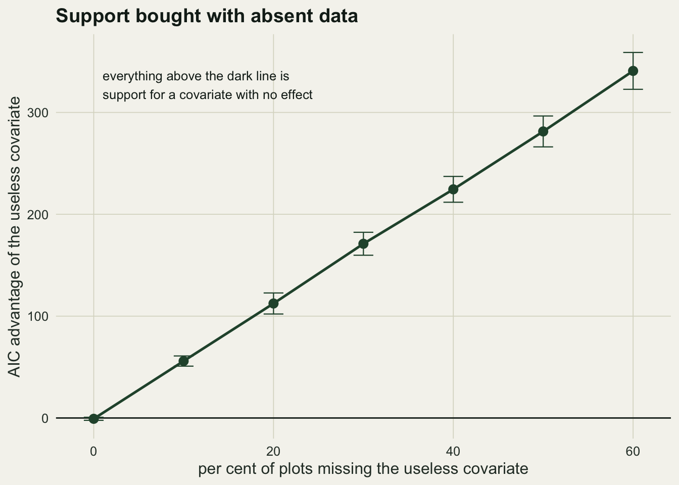
With no missing values at all the true model is ahead by `r sprintf("%.1f", -sw$gap[sw$missing == 0])` AIC units on average: the two-unit penalty for the extra parameter, offset by the improvement in fit a null covariate buys by chance. The elaboration still wins `r sprintf("%.0f", 100 * sw$wrong[sw$missing == 0])` per cent of the time on that margin, which is ordinary AIC behaviour and the reason a gap of one or two units settles nothing.
Then the missingness starts. At a tenth of plots missing the elaboration already wins every one of the `r sw$wrong[sw$missing == 0.1] * 40` simulated data sets, by an average of `r sprintf("%.0f", sw$gap[sw$missing == 0.1])` AIC units. At sixty per cent missing the margin is `r sprintf("%.0f", sw$gap[sw$missing == 0.6])` units in favour of a covariate that does nothing.
```{r fig-sweep}
#| fig-cap: "Mean AIC advantage of a useless covariate over the true model, as a function of how much of that covariate is missing. Forty simulated data sets per point."
#| fig-alt: "A rising curve with error bars, starting slightly below the zero line when nothing is missing and climbing steeply above it, so a covariate with no effect gains hundreds of AIC units of apparent support purely from being missing more often."
ggplot(sw, aes(x = 100 * missing, y = gap)) +
  geom_hline(yintercept = 0, colour = te_ink, linewidth = 0.5) +
  geom_errorbar(aes(ymin = gap - sd, ymax = gap + sd), width = 2.2,
                linewidth = 0.4, colour = te_forest) +
  geom_line(linewidth = 0.9, colour = te_forest) +
  geom_point(size = 2.8, colour = te_forest) +
  annotate("text", x = 1, y = max(sw$gap), hjust = 0, vjust = 1, size = 3.4,
           colour = te_ink,
           label = "everything above the dark line is\nsupport for a covariate with no effect") +
  labs(x = "per cent of plots missing the useless covariate",
       y = "AIC advantage of the useless covariate",
       title = "Support bought with absent data") +
  theme_datasheet()
```
## Making R refuse
The habit that prevents all of this is one line at the top of an analysis script. Setting the default action on missing values to `na.fail` turns the silent drop into an error, so a model that cannot use every row of the frame you handed it stops rather than guessing.
```{r nafail}
old <- options(na.action = "na.fail")
attempt <- try(lm(y ~ x1 + x2, data = plots), silent = TRUE)
cat(class(attempt), ":", conditionMessage(attr(attempt, "condition")), "\n")
options(old)
```
With that set, the workflow becomes: build the analysis frame, subset it to complete cases over every variable in the candidate set, then fit. The models cannot disagree about their data because the frame no longer contains any disagreement.
A lighter check, if you would rather not change a global option, is to compare `nobs` across the fitted models before touching the AIC table. One line, and it catches the whole class.
```{r nobscheck}
same_rows <- function(models) length(unique(sapply(models, nobs))) == 1
c(as_fitted = same_rows(fits), on_common_frame = same_rows(fits_c))
```
## Honest limits
Restricting to complete cases fixes the comparability problem and introduces a different one. It is unbiased only when the values are missing completely at random; when the reason a value is absent is related to the response, dropping those rows biases every estimate in the set, and the tidy AIC table is then a comparison of models fitted to a non-random subsample. Which repair is right depends on why the data are missing, which is not a question the data can answer on their own.
Multiple imputation is the usual alternative, and model selection across imputed data sets is genuinely awkward: the likelihood of an imputed data set is not the likelihood of the observed one, so ordinary AIC does not transfer without modification. That is a real limitation and not a reason to prefer the silent drop, which has no defensible interpretation at all.
The demonstration uses `lm` on a continuous response. The mechanism is the same for `glm` and for mixed models, and in the mixed case there is a second version of the same trap: fits with different fixed-effect structures estimated by restricted maximum likelihood are also not comparable by AIC, for a related reason about what the likelihood is a likelihood of.
Finally, the numbers here belong to one generator with two hundred plots, a moderate effect and independent missingness. The direction of the artefact is general, and the size of it is not; run the sweep on your own frame if you want to know how much of a published ranking could have come from this.
## References
Akaike H 1974 IEEE Transactions on Automatic Control 19(6):716-723 (10.1109/TAC.1974.1100705)
Nakagawa S, Freckleton RP 2008 Trends in Ecology and Evolution 23(11):592-596 (10.1016/j.tree.2008.06.014)
Burnham KP, Anderson DR 2002 Model Selection and Multimodel Inference, 2nd edition, Springer, ISBN 978-0-387-95364-9
## Related tutorials
- [Model selection with AIC](../model-selection-aic/)
- [Missing data mechanisms: MCAR, MAR, MNAR](../missing-data-mechanisms-mcar-mar-mnar/)
- [Akaike weights](../akaike-weights/)
- [Multiple imputation by chained equations](../multiple-imputation-chained-equations/)