set.seed(202)
n  <- 55
moisture <- rnorm(n)
nitrogen <- rnorm(n)
aspect   <- rnorm(n)
biomass  <- 2 + 1.0 * moisture + 0.22 * nitrogen + 0 * aspect + rnorm(n, 0, 1.6)
d <- data.frame(biomass, moisture, nitrogen, aspect)Akaike weights and evidence ratios
R
multimodel inference
model averaging
AIC
ggplot2
ecology tutorial
How to turn AICc differences into Akaike weights and evidence ratios in R, and read variable importance honestly when no single ecological model wins.
Corrected 14 October 2026: a sentence and a figure caption still said that more plots push the weight onto the true model, or concentrate it there; they now say that more plots move more of the weight onto that model but never all of it.
Corrected 7 October 2026: the post put the summed weight of the null aspect term down to its chance inclusion in well-supported models and said such a term can collect a fifth of the weight; it now explains that in a set of all subsets every predictor has a floor on its summed weight, which aspect barely exceeds, so that only a summed weight near one carries a clear message.
Corrected 30 September 2026: the post read four single simulated datasets as showing that the weight keeps concentrating on the true model as evidence accumulates; it now says each point is one noisy draw and that AIC leaves a share of the weight on models with the extra null term however many plots there are.
Model selection in ecology often ends with a table sorted by AIC and a sentence that begins “the best model was”. That sentence hides a question worth asking: how much better was it? Sometimes the top model carries most of the weight and the choice is easy. Just as often two or three models sit within a couple of AIC units of each other, and treating the winner as the truth throws away real uncertainty about which predictors matter.
Akaike weights make that uncertainty explicit. They convert the raw AIC scores of a candidate set into numbers between 0 and 1 that sum to one across the set, so each model gets a share of the evidence rather than a rank. This post builds them by hand from a small grassland example, turns pairs of weights into evidence ratios, and uses the weights to score variable importance, with a warning about how far that last step can be trusted.
If you have not met AIC selection itself yet, fitting several models and comparing them by AIC is the prerequisite; here we take a candidate set as given and ask what to do when no single model stands out.
A candidate set with no clear winner
Fifty-five grassland plots, with log above-ground biomass as the response and three measured predictors: soil moisture, soil nitrogen, and a northness index for slope aspect. Moisture has a clear effect, nitrogen a weak one, and aspect none at all, but a single analysis cannot know that in advance.
With three predictors there are eight possible linear models, from the intercept only up to all three terms. We fit every one and score it with AICc, the small-sample correction to AIC that Burnham and Anderson recommend whenever the ratio of sample size to parameters is small, as it is here.
vars <- c("moisture", "nitrogen", "aspect")
subsets <- unlist(lapply(0:3, function(k) combn(vars, k, simplify = FALSE)),
                  recursive = FALSE)
forms <- vapply(subsets, function(s)
  if (length(s) == 0) "biomass ~ 1" else paste("biomass ~", paste(s, collapse = " + ")),
  character(1))

aicc <- function(m) {
  k <- length(coef(m)) + 1          # slopes + intercept + residual variance
  N <- nobs(m)
  AIC(m) + 2 * k * (k + 1) / (N - k - 1)
}

fits   <- lapply(forms, function(f) lm(as.formula(f), data = d))
scores <- vapply(fits, aicc, numeric(1))
Akaike weights follow from the AICc differences. Subtract the smallest score from each to get the delta values, exponentiate minus half of each delta to get the relative likelihoods, then divide by their total so the set sums to one.
delta <- scores - min(scores)
relL  <- exp(-0.5 * delta)
w     <- relL / sum(relL)

tab <- data.frame(model = forms, dAICc = delta, weight = w)
tab <- tab[order(tab$dAICc), ]
head(tab, 4)
model dAICc weight
5 biomass ~ moisture + nitrogen 0.0000000 0.4465962
2 biomass ~ moisture 0.6675664 0.3198562
8 biomass ~ moisture + nitrogen + aspect 2.4211895 0.1330946
6 biomass ~ moisture + aspect 2.9857938 0.1003594top <- tab[1, ]
second <- tab[2, ]
er_1_2 <- top$weight / second$weight
cum2 <- top$weight + second$weightThe best model, moisture + nitrogen, carries a weight of 0.447. That is the largest share, but it is not a majority: the second model, moisture, sits only 0.67 AICc units behind with a weight of 0.320. Together the top two account for 77 per cent of the evidence, and the difference between them comes down to whether the weak nitrogen term earns its place. This is exactly the situation where reporting only the winner would overstate what the data can support.
Evidence ratios
The ratio of two Akaike weights is an evidence ratio: how many times more support the data give one model over another. It reads more naturally than a delta value because it is a plain multiple.
er_best_null <- top$weight / tab$weight[tab$model == "biomass ~ 1"]Here the best model is favoured over the second by a factor of only 1.40. A ratio that close to one is the quantitative version of “these two models are hard to tell apart”, and it is a far more honest summary than declaring a single winner. For contrast, the best model beats the intercept-only model by a factor of 11484, so the predictors as a group clearly carry signal even though the choice among them is unsettled.
A rough convention treats evidence ratios below about 2 or 3 as weak, and ratios in the tens or hundreds as strong. The point of the number is not the threshold but the scale: it tells you whether the ranking is decisive or a coin toss dressed up as a decision.
Variable importance from summed weights
Because the weights sum to one across the set, you can ask a different question of them: for each predictor, add up the weights of every model that contains it. This sum of weights, written w+, is often read as the relative importance of that predictor.
importance <- vapply(vars, function(v) {
  in_model <- vapply(subsets, function(s) v %in% s, logical(1))
  sum(w[in_model])
}, numeric(1))
importance
moisture nitrogen aspect
0.9999065 0.5797313 0.2334785 imp_moist <- importance["moisture"]
imp_nitro <- importance["nitrogen"]
imp_aspect <- importance["aspect"]
# the least w+ any predictor can collect in this set: each model containing it
# has a partner without it (2 to 4 parameters) that it can beat only on fit
pen <- function(k) 2 * k + 2 * k * (k + 1) / (n - k - 1) # AICc penalty
step_max <- max(pen(3:5) - pen(2:4))
wplus_min <- exp(-step_max / 2) / (1 + exp(-step_max / 2))Moisture appears in every well-supported model and reaches w+ = 1.00. Nitrogen, the weak real effect, lands at 0.58. Aspect, which has no effect at all, still collects w+ = 0.23, and that is barely more than the least any predictor can collect in this set: every model with aspect has a partner without it that differs only by that one term, and the AICc penalty for one extra parameter is modest, so each model with aspect keeps at least a fixed share of its partner’s weight even when aspect explains nothing.
That last number is the catch. A predictor unrelated to the response does not get w+ near zero; in a candidate set of all subsets it cannot fall below 0.23 here, and over repeated datasets it often lands higher. Galipaud and colleagues showed that w+ takes a wide range of values even for pure noise predictors, so a middling w+ cannot be read as evidence that a variable matters. Only a w+ near one carries a clear message; the middle, which in a set of all subsets starts at that floor, is ambiguous.
library(ggplot2)
te_canvas <- theme(plot.background  = element_rect(fill = "#f5f4ee", colour = NA),
                   panel.background = element_rect(fill = "#f5f4ee", colour = NA))
impdf <- data.frame(predictor = names(importance), wplus = as.numeric(importance))
impdf$predictor <- factor(impdf$predictor, levels = impdf$predictor[order(impdf$wplus)])

thumb_tab <- head(tab, 5)
thumb_tab$mod <- gsub("biomass ~ ", "", thumb_tab$model)
thumb_tab$mod <- factor(thumb_tab$mod, levels = rev(thumb_tab$mod))
p_thumb <- ggplot(thumb_tab, aes(weight, mod)) +
  geom_segment(aes(x = 0, xend = weight, yend = mod), colour = "#adbcd9") +
  geom_point(colour = "#4c72b0", size = 4) +
  scale_x_continuous(limits = c(0, NA), expand = expansion(mult = c(0, 0.08))) +
  labs(title = paste(strwrap("Akaike weight by candidate model", 46), collapse = "\n"),
       x = "Akaike weight", y = NULL) +
  theme_minimal(base_size = 12) + te_canvas +
  theme(plot.title = element_text(size = 13, face = "bold"),
        plot.subtitle = element_text(size = 9.5),
        plot.margin = margin(8, 14, 8, 8))

ggplot(impdf, aes(wplus, predictor)) +
  geom_col(fill = "#4c72b0", width = 0.6) +
  geom_vline(xintercept = 0.5, linetype = "dashed", colour = "grey55") +
  scale_x_continuous(limits = c(0, 1), expand = expansion(mult = c(0, 0.02))) +
  labs(x = "summed Akaike weight (w+)", y = NULL) +
  theme_minimal(base_size = 12) + te_canvas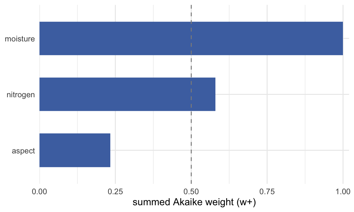
How the weights sharpen with sample size
None of this is fixed. The same three effects, measured on more plots, move more of the weight onto the model that matches the truth, though never all of it; measured on fewer, the weight spreads out because the data cannot separate close models. The plot below repeats the whole selection at four sample sizes and tracks the weight landing on the two-predictor model that contains both real effects.
weight_target <- function(N, seed = 202) {
  set.seed(seed)
  mo <- rnorm(N); ni <- rnorm(N); as <- rnorm(N)
  bm <- 2 + 1.0 * mo + 0.22 * ni + 0 * as + rnorm(N, 0, 1.6)
  dd <- data.frame(bm, mo, ni, as)
  vv <- c("mo", "ni", "as")
  ss <- unlist(lapply(0:3, function(k) combn(vv, k, simplify = FALSE)), recursive = FALSE)
  ff <- vapply(ss, function(s)
    if (length(s) == 0) "bm ~ 1" else paste("bm ~", paste(s, collapse = " + ")), character(1))
  sc <- vapply(lapply(ff, function(f) lm(as.formula(f), data = dd)), aicc, numeric(1))
  ww <- exp(-0.5 * (sc - min(sc))); ww <- ww / sum(ww)
  target <- vapply(ss, function(s) setequal(s, c("mo", "ni")), logical(1))
  sum(ww[target])
}
ns <- c(30, 55, 120, 400)
wn <- vapply(ns, weight_target, numeric(1))
ndf <- data.frame(n = ns, weight = wn)
ggplot(ndf, aes(n, weight)) +
  geom_line(colour = "#4c72b0") +
  geom_point(colour = "#4c72b0", size = 2) +
  scale_x_continuous(breaks = ns) +
  scale_y_continuous(limits = c(0, 1)) +
  labs(x = "number of plots", y = "weight on moisture + nitrogen model") +
  theme_minimal(base_size = 12) + te_canvas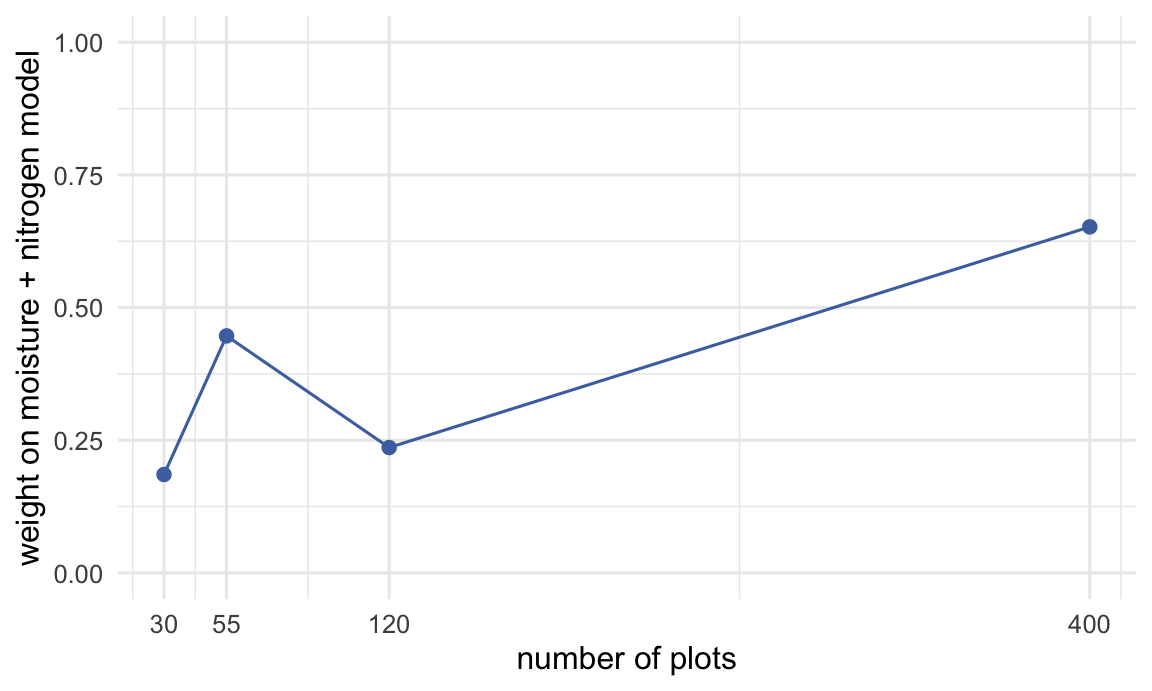
w_small <- wn[1]
w_big   <- wn[length(wn)]
At thirty plots the target model holds only 0.185 of the weight; at four hundred it reaches 0.652. The path is not perfectly smooth, because each point is a single simulated dataset, and the rise does not carry on towards one: AIC keeps giving a share of the weight to the models that add the null aspect term however many plots there are, so averaged over many simulated datasets the weight on the moisture-plus-nitrogen model levels off well short of one. More plots separate the models with real effects from those without, but they do not make AIC single out the true model. When your weights are spread thin, that is the data telling you the candidate models are genuinely close, not a defect to be optimised away.
What the weights do and do not settle
Akaike weights turn a ranked table into a statement about evidence, and evidence ratios make the comparison between any two models a single interpretable multiple. Both are honest about ambiguity in a way that “the best model was” is not. Summed weights are more fragile: they answer “how much of the supported model space includes this predictor”, which is only loosely related to whether the predictor has an effect, and they should never be the sole basis for claiming importance.
The weights raise an obvious next question. If several models share the evidence, why commit to one at all for prediction or for effect sizes? That is what model averaging addresses, and it splits into a safe path and a treacherous one depending on whether you average predictions or coefficients.
References
Burnham KP, Anderson DR 2002 Model Selection and Multimodel Inference: A Practical Information-Theoretic Approach, 2nd ed. Springer, New York. ISBN 978-0-387-95364-9
Symonds MRE, Moussalli A 2011 Behavioral Ecology and Sociobiology 65(1):13-21 (10.1007/s00265-010-1037-6)
Burnham KP, Anderson DR, Huyvaert KP 2011 Behavioral Ecology and Sociobiology 65(1):23-35 (10.1007/s00265-010-1029-6)
Galipaud M, Gillingham MAF, David M, Dechaume-Moncharmont FX 2014 Methods in Ecology and Evolution 5(10):983-991 (10.1111/2041-210X.12251)