Model-averaged predictions

Why model-averaged predictions beat picking one best model in R: an unconditional interval that accounts for selection uncertainty and covers correctly.

Once a candidate set shares its Akaike weight across several models, committing to the single best one for prediction quietly discards the fact that other models fit almost as well and sometimes predict something different. Model averaging offers a way out that, for predictions specifically, is both simple and well behaved: take each model’s prediction at the site you care about and combine them in proportion to their weights.

The payoff is not a better point estimate so much as an honest interval. A prediction interval from the best model conditions on that model being correct, which it is not; the model-averaged interval widens to absorb the disagreement among models, and as a result it covers the truth at close to its nominal rate. This post builds the averaged prediction and its unconditional interval by hand, then checks the coverage by simulation.

The Akaike weights post is the prerequisite; here the weights are the tool rather than the topic.

A prediction at a new plot

The same fifty-five grassland plots as before, with log above-ground biomass predicted from soil moisture, nitrogen, and a northness index. We want the prediction at a new plot that is wet and nitrogen-rich with a pronounced aspect: moisture and nitrogen one standard deviation above average, aspect two.

set.seed(303)
n  <- 55
moisture <- rnorm(n); nitrogen <- rnorm(n); aspect <- rnorm(n)
biomass  <- 2 + 1.0 * moisture + 0.22 * nitrogen + 0 * aspect + rnorm(n, 0, 1.6)
d <- data.frame(biomass, moisture, nitrogen, aspect)

vars    <- c("moisture", "nitrogen", "aspect")
subsets <- unlist(lapply(0:3, function(k) combn(vars, k, simplify = FALSE)), recursive = FALSE)
forms   <- vapply(subsets, function(s)
  if (length(s) == 0) "biomass ~ 1" else paste("biomass ~", paste(s, collapse = " + ")), character(1))
aicc <- function(m) { k <- length(coef(m)) + 1; N <- nobs(m); AIC(m) + 2 * k * (k + 1) / (N - k - 1) }

fits  <- lapply(forms, function(f) lm(as.formula(f), data = d))
w     <- exp(-0.5 * (vapply(fits, aicc, numeric(1)) - min(vapply(fits, aicc, numeric(1)))))
w     <- w / sum(w)

newplot  <- data.frame(moisture = 1, nitrogen = 1, aspect = 2)
true_mean <- 2 + 1.0 * 1 + 0.22 * 1 + 0 * 2

The true mean at this plot is 3.22, though in a real analysis you would not know it. Each of the eight models produces its own prediction there, together with a standard error for that prediction.

pred <- t(vapply(fits, function(m) {
  p <- predict(m, newplot, se.fit = TRUE)
  c(fit = as.numeric(p$fit), se = as.numeric(p$se.fit))
}, numeric(2)))
pred <- as.data.frame(pred)
pred$weight <- w
range_fit <- range(pred$fit)

The point predictions range from 1.69 to 3.35 depending on which model you trust, a spread of 1.66 on the log-biomass scale. That spread is the selection uncertainty a single best model would hide.

The best-model interval

Selecting the top model and reporting its prediction interval is the usual shortcut.

best_i  <- which.max(w)
pb      <- predict(fits[[best_i]], newplot, se.fit = TRUE)
tcrit   <- qt(0.975, fits[[best_i]]$df.residual)
best_lo <- as.numeric(pb$fit) - tcrit * pb$se.fit
best_hi <- as.numeric(pb$fit) + tcrit * pb$se.fit

The best model predicts 3.16, with a 95 per cent interval from 2.46 to 3.86, a width of 1.40. This interval is conditional: it describes the uncertainty assuming the chosen model is the right one, and says nothing about the chance that a different model, fitting nearly as well, would have placed the prediction elsewhere.

The model-averaged interval

The averaged prediction is the weighted mean of the eight point predictions. Its standard error has to combine two sources of uncertainty: the ordinary within-model error of each prediction, and the between-model variation in where the models place the point. The unconditional standard error of Burnham and Anderson does exactly this, weighting each model’s contribution by its Akaike weight.

y_avg  <- sum(w * pred$fit)
se_unc <- sum(w * sqrt(pred$se^2 + (pred$fit - y_avg)^2))
avg_lo <- y_avg - 1.96 * se_unc
avg_hi <- y_avg + 1.96 * se_unc

The model-averaged prediction is 3.10, close to the best-model value, but its 95 per cent interval runs from 2.27 to 3.94, a width of 1.67. The extra width is the between-model term: the models disagree about the prediction at this plot, and the unconditional interval refuses to pretend otherwise.

library(ggplot2)
pd <- pred[order(pred$fit), ]
pd$rank <- seq_len(nrow(pd))
ggplot(pd, aes(fit, rank)) +
  geom_vline(xintercept = true_mean, linetype = "dashed", colour = "grey55") +
  geom_point(aes(size = weight), colour = "grey35", alpha = 0.8) +
  geom_point(aes(x = y_avg, y = max(rank) + 1), colour = "#4c72b0", size = 3) +
  geom_errorbarh(aes(xmin = avg_lo, xmax = avg_hi, y = max(rank) + 1),
                 height = 0.4, colour = "#4c72b0") +
  scale_size(range = c(1.5, 6), guide = "none") +
  scale_y_continuous(breaks = NULL) +
  labs(x = "predicted log biomass at new plot", y = NULL,
       subtitle = "grey: candidate models (size = weight); blue: model-averaged with unconditional interval") +
  theme_minimal(base_size = 12)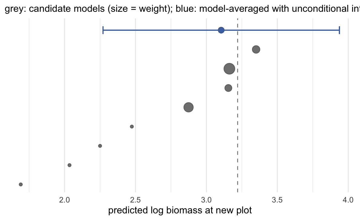

Warning: `geom_errorbarh()` was deprecated in ggplot2 4.0.0.
ℹ Please use the `orientation` argument of `geom_errorbar()` instead.

Warning in geom_point(aes(x = y_avg, y = max(rank) + 1), colour = "#4c72b0", : All aesthetics have length 1, but the data has 8 rows.
ℹ Please consider using `annotate()` or provide this layer with data containing
  a single row.

`height` was translated to `width`.

Figure 1: Predictions from the eight candidate models at the new plot, point size scaled by Akaike weight. The model-averaged value (blue) and its unconditional interval sit near the well-supported models; the true mean (dashed) falls inside.

Does the wider interval actually cover?

A wider interval is only better if the extra width buys accurate coverage rather than needless conservatism. The test is a simulation: generate many datasets from the same truth, build both intervals each time, and count how often each contains the true mean at the new plot. A well-calibrated 95 per cent interval should cover about 95 per cent of the time.

cover_sim <- function(reps = 2000, seed = 3033) {
  set.seed(seed)
  cb <- wb <- ca <- wa <- 0
  np <- data.frame(moisture = 1, nitrogen = 1, aspect = 2)
  for (i in seq_len(reps)) {
    moisture <- rnorm(n); nitrogen <- rnorm(n); aspect <- rnorm(n)
    biomass  <- 2 + 1.0 * moisture + 0.22 * nitrogen + 0 * aspect + rnorm(n, 0, 1.6)
    dd <- data.frame(biomass, moisture, nitrogen, aspect)
    fj <- lapply(forms, function(f) lm(as.formula(f), data = dd))
    sj <- vapply(fj, aicc, numeric(1)); wj <- exp(-0.5 * (sj - min(sj))); wj <- wj / sum(wj)
    fj_fit <- vapply(fj, function(m) as.numeric(predict(m, np)), numeric(1))
    fj_se  <- vapply(fj, function(m) as.numeric(predict(m, np, se.fit = TRUE)$se.fit), numeric(1))
    bi <- which.max(wj); tb <- qt(0.975, fj[[bi]]$df.residual)
    lo <- fj_fit[bi] - tb * fj_se[bi]; hi <- fj_fit[bi] + tb * fj_se[bi]
    cb <- cb + (true_mean >= lo && true_mean <= hi); wb <- wb + (hi - lo)
    ya <- sum(wj * fj_fit); su <- sum(wj * sqrt(fj_se^2 + (fj_fit - ya)^2))
    la <- ya - 1.96 * su; ha <- ya + 1.96 * su
    ca <- ca + (true_mean >= la && true_mean <= ha); wa <- wa + (ha - la)
  }
  c(cover_best = cb / reps, width_best = wb / reps,
    cover_avg = ca / reps, width_avg = wa / reps)
}
cov <- cover_sim()
cov

cover_best width_best  cover_avg  width_avg 
  0.872500   1.452636   0.961000   1.876228 

cb <- cov["cover_best"]; ca <- cov["cover_avg"]
wbst <- cov["width_best"]; wavg <- cov["width_avg"]

The best-model interval covers the truth 87.2 per cent of the time, well below its nominal 95, with a mean width of 1.45. The model-averaged interval covers 96.1 per cent, essentially on target, at a mean width of 1.88. The averaged interval is wider, but the extra width is doing real work: it restores the coverage that model selection had silently eaten. Reporting the best-model interval here would understate uncertainty by enough to matter.

covdf <- data.frame(method = c("best model", "model-averaged"),
                    coverage = c(cb, ca) * 100)
ggplot(covdf, aes(method, coverage, fill = method)) +
  geom_col(width = 0.6) +
  geom_hline(yintercept = 95, linetype = "dashed", colour = "grey40") +
  scale_fill_manual(values = c("best model" = "grey55", "model-averaged" = "#4c72b0"),
                    guide = "none") +
  coord_cartesian(ylim = c(80, 100)) +
  labs(x = NULL, y = "coverage of 95% interval (%)") +
  theme_minimal(base_size = 12)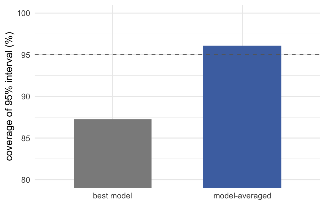

Figure 2: Coverage of nominal 95 per cent prediction intervals over 2000 simulated datasets. The best-model interval undercovers; the model-averaged interval reaches its nominal rate.

When this works, and one caveat

Averaging predictions is the safe face of model averaging. Each model produces a prediction on the same scale, the weighted mean of those predictions is a sensible quantity, and the unconditional interval turns model disagreement into honest width. Nothing here required the models to be nested or to share a common parameterisation.

One caveat matters for non-linear models. For a generalised linear model with a link function, you must average the predictions on the response scale, after applying the inverse link to each model, not average linear-predictor coefficients and transform once. Averaging on the wrong scale reintroduces exactly the problem this method avoids. Grueber and colleagues, whose appendix on averaged prediction intervals was later corrected for producing intervals that were too wide, are worth reading alongside Burnham and Anderson on this point.

The reason predictions average cleanly while coefficients do not is worth its own treatment, because the coefficient version is where model averaging most often goes wrong in the ecological literature.

Related tutorials

• Akaike weights and evidence ratios
• Model-averaged coefficients: a caution
• Conformal prediction intervals
• Checking a multi-model analysis

References

Burnham KP, Anderson DR (2002) Model Selection and Multimodel Inference: A Practical Information-Theoretic Approach, 2nd ed. Springer, New York. ISBN 978-0-387-95364-9

Grueber CE, Nakagawa S, Laws RJ, Jamieson IG (2011) Journal of Evolutionary Biology 24(4):699-711 (10.1111/j.1420-9101.2010.02210.x)