gen_data <- function(rho, N = 80, seed = 505) {
  if (!is.na(seed)) set.seed(seed)          # seed = NA gives a fresh draw each call
  z1 <- rnorm(N); z2 <- rnorm(N)
  moisture <- z1
  carbon   <- rho * z1 + sqrt(1 - rho^2) * z2   # correlation with moisture = rho
  aspect   <- rnorm(N)
  biomass  <- 2 + 1.0 * moisture + 1.4 * carbon + 0 * aspect + rnorm(N, 0, 2.0)
  data.frame(biomass, moisture, carbon, aspect)
}Model-averaged coefficients: a caution
R
multimodel inference
model averaging
collinearity
ggplot2
ecology tutorial
Model-averaged regression coefficients mislead under collinearity in ecology (Cade 2015). Average predictions, not coefficients: a worked R demonstration.
Corrected 14 October 2026: the post said that averaging predictions is safe and that the coefficient problem never touches a prediction; in a linear model the averaged prediction is the full average of each coefficient applied to the site, so this holds only at sites that follow the correlation in the data, and the text now says so throughout.
Corrected 7 October 2026: the post said the candidate models agree about the total prediction at any given site; they agree only where moisture and carbon rise together as they do in strongly correlated data, as at the site checked here, and the text now says so.
Updated 27 September 2026: a new section, Full and conditional averages, measures how far apart the two model-averaged coefficients sit on this post’s candidate set, and which of them MuMIn’s coef() and predict() use by default.
Averaging predictions across a candidate set is safe at sites that follow the correlation in the data. Averaging coefficients across the same set is where multi-model inference most often goes wrong in ecology, and it goes wrong precisely when it looks most useful: when predictors are correlated and you want a single number for each one’s effect.
The problem is not a coding slip. It is that a regression coefficient means different things in different models. In a model that also contains a correlated predictor, a coefficient is a partial effect, holding that other predictor fixed. In a model that omits it, the same coefficient absorbs the shared variation and becomes something larger. Averaging those two numbers, weighted by Akaike weights, blends quantities that are not on the same footing. Cade set this out in detail in 2015; this post reproduces the core of the argument in R and shows why the prediction at a site that follows the correlation stays trustworthy even as the averaged coefficient does not.
The Akaike weights post is the prerequisite, and the collinearity and variance inflation post covers the mechanism this one builds on.
Partial, marginal and averaged on one dataset
Take a single dataset with strong correlation, and estimate the moisture coefficient two ways: from the model that also includes carbon (a partial effect), and from the model with moisture alone (a marginal effect).
d09 <- gen_data(rho = 0.9)
b_partial  <- coef(lm(biomass ~ moisture + carbon, data = d09))["moisture"]
b_marginal <- coef(lm(biomass ~ moisture, data = d09))["moisture"]
c(partial = as.numeric(b_partial), marginal = as.numeric(b_marginal))
partial marginal
0.6885105 2.5707228 The partial effect is 0.69; the marginal is 2.57. With carbon left out the moisture term stands in for both gradients at once. Any single fit is a noisy draw, especially with strong collinearity inflating its standard error; the systematic behaviour comes from averaging over many datasets, which we do shortly. Neither estimate is wrong for what it is, they simply answer different questions, and a model-averaged coefficient mixes them.
To see the averaged coefficient itself, we need the full candidate set. With three predictors there are eight models; the averaged moisture coefficient adds up each model’s moisture estimate weighted by its Akaike weight, counting models without moisture as contributing zero.
aicc <- function(m) { k <- length(coef(m)) + 1; N <- nobs(m); AIC(m) + 2 * k * (k + 1) / (N - k - 1) }
vars <- c("moisture", "carbon", "aspect")
subsets <- unlist(lapply(0:3, function(k) combn(vars, k, simplify = FALSE)), recursive = FALSE)
forms   <- vapply(subsets, function(s)
  if (length(s) == 0) "biomass ~ 1" else paste("biomass ~", paste(s, collapse = " + ")), character(1))

avg_moisture <- function(d) {
  fits <- lapply(forms, function(f) lm(as.formula(f), data = d))
  w <- exp(-0.5 * (vapply(fits, aicc, numeric(1)) - min(vapply(fits, aicc, numeric(1)))))
  w <- w / sum(w)
  b <- vapply(fits, function(m) { cc <- coef(m); if ("moisture" %in% names(cc)) cc["moisture"] else 0 }, numeric(1))
  in_m <- vapply(subsets, function(s) "moisture" %in% s, logical(1))
  c(avg_coef = sum(w * b), wplus = sum(w[in_m]))
}
avg_moisture(d09)
avg_coef wplus
0.3098513 0.3927900 Watching the marginal estimate drift with collinearity
The single dataset is suggestive, but the honest claim is about expected behaviour, so we repeat the whole exercise across a range of correlations, averaging over many datasets at each level to smooth out the noise. At each correlation we record the partial estimate, the marginal estimate, the model-averaged estimate, the summed weight for moisture, and, as a check, the model-averaged prediction at a fixed site.
one_rep <- function(rho) {
  d <- gen_data(rho, seed = NA)
  fits <- lapply(forms, function(f) lm(as.formula(f), data = d))
  w <- exp(-0.5 * (vapply(fits, aicc, numeric(1)) - min(vapply(fits, aicc, numeric(1)))))
  w <- w / sum(w)
  in_m <- vapply(subsets, function(s) "moisture" %in% s, logical(1))
  bm <- vapply(fits, function(m) { cc <- coef(m); if ("moisture" %in% names(cc)) cc["moisture"] else 0 }, numeric(1))
  x0 <- data.frame(moisture = 1, carbon = 1, aspect = 0)
  c(partial  = as.numeric(coef(fits[[which(forms == "biomass ~ moisture + carbon")]])["moisture"]),
    marginal = as.numeric(coef(fits[[which(forms == "biomass ~ moisture")]])["moisture"]),
    averaged = sum(w * bm),
    wplus    = sum(w[in_m]),
    pred     = sum(w * vapply(fits, function(m) as.numeric(predict(m, x0)), numeric(1))))
}

rhos <- c(0, 0.3, 0.6, 0.9)
set.seed(505)
sweep <- t(vapply(rhos, function(r) {
  colMeans(t(vapply(seq_len(300), function(i) one_rep(r), numeric(5))))
}, numeric(5)))
sweep <- data.frame(rho = rhos, sweep)
round(sweep, 3)
rho partial marginal averaged wplus pred
1 0.0 0.991 0.963 0.980 0.980 4.386
2 0.3 1.014 1.429 1.001 0.976 4.398
3 0.6 1.005 1.825 0.972 0.942 4.386
4 0.9 1.025 2.274 0.929 0.674 4.398lo <- sweep[sweep$rho == 0, ]
hi <- sweep[sweep$rho == 0.9, ]At near-zero correlation, all three coefficient estimates agree near the true 1.0 and the summed weight for moisture sits at 0.98. As the correlation climbs to 0.9, the partial estimate stays put at 1.02, but the marginal estimate inflates to 2.27, and the model-averaged estimate sits at 0.93 as the weight shifts among models that mean different things by “moisture”. The summed weight for moisture, meanwhile, falls from 0.98 to 0.67, which would read as moisture becoming less important even though its true effect never changed.
library(ggplot2)
te_canvas <- theme(plot.background  = element_rect(fill = "#f5f4ee", colour = NA),
                   panel.background = element_rect(fill = "#f5f4ee", colour = NA))
long <- data.frame(
  rho = rep(sweep$rho, 3),
  estimate = c(sweep$partial, sweep$marginal, sweep$averaged),
  kind = rep(c("partial (with carbon)", "marginal (moisture only)", "model-averaged"), each = nrow(sweep)))
ggplot(long, aes(rho, estimate, colour = kind)) +
  geom_hline(yintercept = 1.0, linetype = "dashed", colour = "grey55") +
  geom_line(linewidth = 0.8) + geom_point(size = 2) +
  scale_colour_manual(values = c("partial (with carbon)" = "#4c72b0",
                                 "marginal (moisture only)" = "#c44e52",
                                 "model-averaged" = "#55a868"), name = NULL) +
  labs(x = "correlation between moisture and carbon", y = "estimated moisture coefficient") +
  theme_minimal(base_size = 12) + te_canvas + theme(legend.position = "top")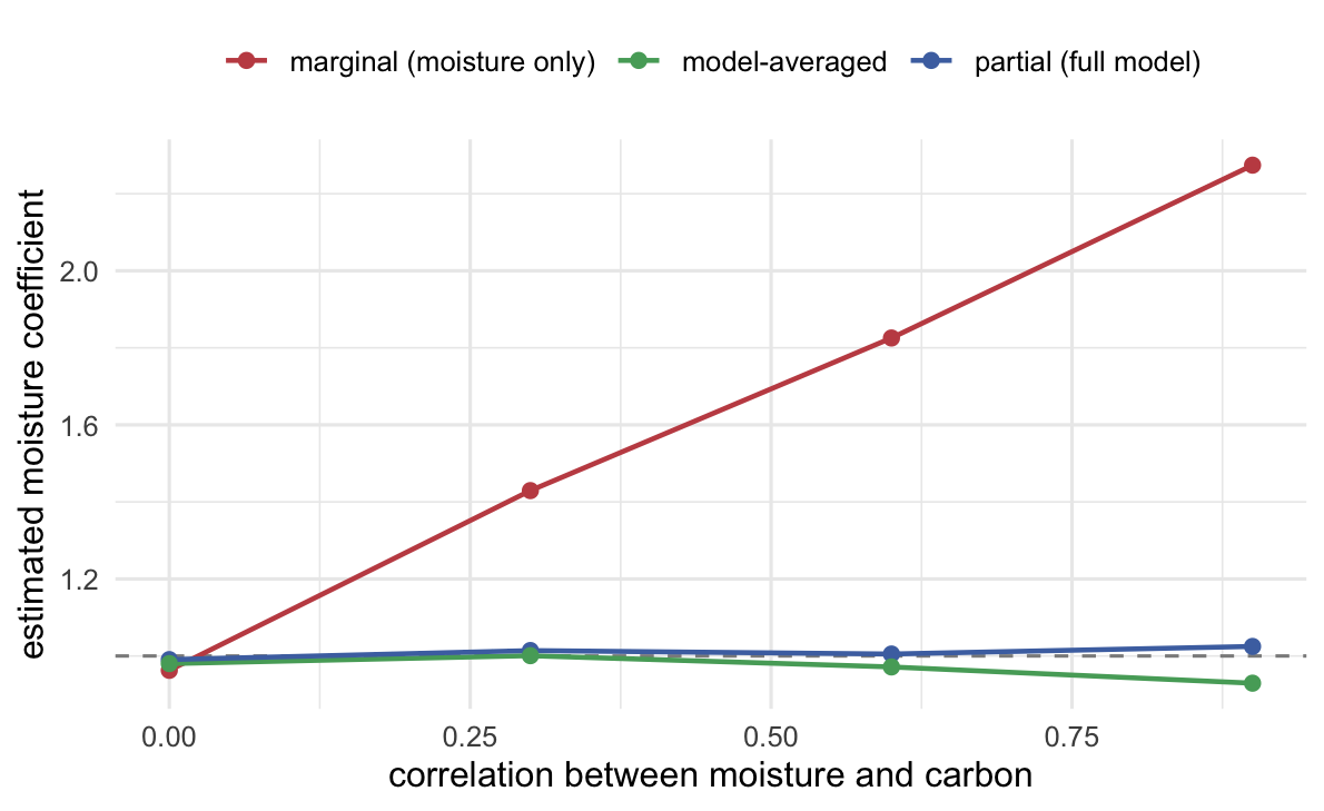
The prediction is fine the whole time
Here is the reassuring half. The same candidate set, averaged the same way, gives a model-averaged prediction that barely moves as collinearity increases. The models disagree about how to split the effect between moisture and carbon, but at a site like the one checked here, where moisture and carbon rise together as they do in strongly correlated data, they agree about the total.
ggplot(sweep, aes(rho, pred)) +
  geom_hline(yintercept = 4.4, linetype = "dashed", colour = "grey55") +
  geom_line(colour = "#4c72b0", linewidth = 0.8) + geom_point(colour = "#4c72b0", size = 2) +
  coord_cartesian(ylim = c(3.8, 5.0)) +
  labs(x = "correlation between moisture and carbon", y = "model-averaged prediction at site") +
  theme_minimal(base_size = 12) + te_canvas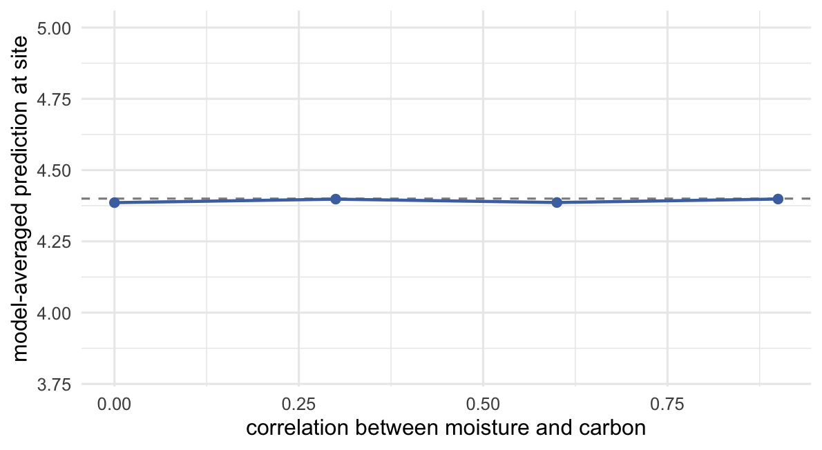
Full and conditional averages
Every averaged coefficient so far is a full average: a model without moisture enters with a coefficient of zero. The other common recipe, the conditional average, takes the weighted mean over only the models that contain the term, with their weights rescaled to sum to one among them. Grueber and colleagues describe the two as the zero method and the natural average. They are tied by an identity, full = w+ x conditional, so they agree only when the summed weight is one. Which one ends up in a results table can come down to a software default. In the MuMIn package (version 1.48.19, read from its source; it is not loaded here), summary() of a model average prints both, labelled “(full average)” and “(conditional average)”, but coef() and confint() default to full = FALSE, the conditional one, while predict() defaults to full = TRUE.
global <- lm(biomass ~ moisture + carbon + aspect, data = d09, na.action = na.fail)
ms  <- MuMIn::dredge(global)              # the same eight models, ranked by AICc
avg <- MuMIn::model.avg(ms, subset = delta < 2)
coef(avg)                                 # conditional average: the default
coef(avg, full = TRUE)                    # full average over the delta < 2 set (top_full below)
The next chunk computes both averages over all eight models and over the models within 2 AICc units of the best (the common “delta < 2” set, weights rescaled within it), checks the identity and the post’s own average on the single data set from above, then repeats the collinearity sweep with its own seed.
with_c <- vapply(subsets, function(s) "carbon" %in% s, logical(1))
ca_avg <- function(d, term) {
  fits <- lapply(forms, function(f) lm(as.formula(f), data = d))
  a <- vapply(fits, aicc, numeric(1)); dl <- a - min(a)
  b <- vapply(fits, function(m) { cc <- coef(m); if (term %in% names(cc)) cc[[term]] else 0 }, numeric(1))
  has <- vapply(subsets, function(s) term %in% s, logical(1))
  out <- c()
  for (keep in list(rep(TRUE, 8), dl < 2)) {
    w <- exp(-dl / 2) * keep; w <- w / sum(w); wp <- sum(w[has])
    out <- c(out, sum(w * b), if (wp > 0) sum(w * b) / wp else NA, wp, sum(w[has & !with_c]) / wp)
  }
  names(out) <- paste(rep(c("all", "top"), each = 4), c("full", "cond", "wplus", "nocarbon"), sep = "_")
  c(out, ols = b[8], ols_se = coef(summary(fits[[8]]))[term, 2])
}
ca_d09 <- ca_avg(d09, "moisture")
stopifnot(all.equal(ca_d09[["all_full"]], avg_moisture(d09)[["avg_coef"]]),
          all.equal(ca_d09[["all_full"]], ca_d09[["all_wplus"]] * ca_d09[["all_cond"]]),
          all.equal(ca_d09[["top_full"]], ca_d09[["top_wplus"]] * ca_d09[["top_cond"]]))
set.seed(353)
ca_runs <- lapply(rhos, function(r) t(replicate(400, ca_avg(gen_data(r, seed = NA), "moisture"))))
ca_rho <- data.frame(rho = rhos, t(vapply(ca_runs, colMeans, numeric(10), na.rm = TRUE)))
round(ca_rho[, c("rho", "all_full", "all_cond", "top_full", "top_cond", "ols")], 3)
rho all_full all_cond top_full top_cond ols
1 0.0 0.989 1.000 0.996 1.000 1.000
2 0.3 0.981 0.996 0.991 0.996 0.995
3 0.6 0.977 1.013 0.994 1.010 1.010
4 0.9 0.921 1.130 0.930 1.162 0.989ca_gap_se <- sd(ca_runs[[4]][, "all_cond"] - ca_runs[[4]][, "all_full"]) / sqrt(400)At no correlation the two averages differ by 0.010 and both sit on the true 1.0. At a correlation of 0.9 they part: over all eight models the full average of moisture is 0.92 and the conditional average 1.13, a gap of 0.21 (Monte Carlo SE 0.008), and the delta < 2 set gives 0.93 and 1.16 (the latter over the 92 per cent of data sets in which moisture stays in the set), while the full-model estimate averages 0.99. So at high collinearity the number coef() prints on this candidate set is not the value drawn in the first figure, which is the full average. The conditional average is a weighted mean over the four models that contain moisture, and the two of them without carbon, whose moisture coefficient is the marginal one (2.27 at this correlation in the sweep above), hold on average 18 per cent of that weight; in each data set the full average is the conditional one times the summed weight, which averages 0.68 here. The averages do not multiply (0.77 against 0.92), because the summed weight and the conditional average rise and fall together across data sets (correlation 0.92).
The two averages also part without any collinearity. The next chunk goes back to independent predictors (correlation 0) and gives aspect a weak real effect b, added to the post’s own generator, with 1000 data sets per value of b.
ca_b <- c(0, 0.15, 0.25, 0.4)
set.seed(354)
ca_weak <- lapply(ca_b, function(bw) t(replicate(1000, {
  d <- gen_data(0, seed = NA); d$biomass <- d$biomass + bw * d$aspect
  ca_avg(d, "aspect") })))
ca_tab <- data.frame(b = ca_b, t(vapply(seq_along(ca_b), function(i) {
  r <- ca_weak[[i]]; bw <- ca_b[i]; kept <- !is.na(r[, "top_cond"])
  rmse <- function(x) sqrt(mean((x - bw)^2))
  rmse_se <- function(x) sd((x - bw)^2) / sqrt(length(x)) / (2 * rmse(x))
  c(top_cond = mean(r[kept, "top_cond"]), top_full = mean(r[, "top_full"]),
    all_cond = mean(r[, "all_cond"]), ols = mean(r[, "ols"]), ols_kept = mean(r[kept, "ols"]),
    rmse_cond = rmse(r[kept, "top_cond"]), rmse_full = rmse(r[, "top_full"]), rmse_ols = rmse(r[, "ols"]),
    rmse_ols_kept = rmse(r[kept, "ols"]), rmse_full_kept = rmse(r[kept, "top_full"]), absent = mean(!kept), se_cond = sd(r[kept, "top_cond"]) / sqrt(sum(kept)),
    se_full = sd(r[, "top_full"]) / sqrt(nrow(r)), ols_se = mean(r[, "ols_se"]),
    rmse_se = max(rmse_se(r[kept, "top_cond"]), rmse_se(r[, "top_full"])))
}, numeric(15))))
round(ca_tab[, c("b", "top_cond", "top_full", "all_cond", "ols", "absent", "rmse_cond", "rmse_full", "rmse_ols")], 3)
b top_cond top_full all_cond ols absent rmse_cond rmse_full rmse_ols
1 0.00 -0.004 0.001 -0.003 -0.003 0.388 0.292 0.154 0.232
2 0.15 0.216 0.097 0.153 0.152 0.306 0.256 0.183 0.230
3 0.25 0.306 0.166 0.243 0.243 0.222 0.229 0.229 0.231
4 0.40 0.446 0.323 0.394 0.394 0.124 0.216 0.283 0.242ca_null <- ca_weak[[1]]
ca_pc <- function(col, i) 100 * (ca_tab[i, col] / ca_b[i] - 1)The full-model standard error of the aspect coefficient is about 0.23, so b = 0.15 is 0.65 of a standard error and b = 0.4 is 1.75. With b = 0.15, aspect drops out of the delta < 2 set in 31 per cent of data sets, which leaves no conditional estimate at all. Where it stays, the conditional average is 0.216, 44 per cent too large (Monte Carlo SE 6 percentage points), and the full average over the delta < 2 set, which is zero where aspect was dropped, averages 0.097 over all data sets, 36 per cent too small (Monte Carlo SE 4 percentage points). The inflation is selection: in the data sets that keep aspect, the full-model estimate itself averages 0.215, against 0.152 over all data sets, the winner’s curse of checking a multi-model analysis. Over all eight models, where no model is dropped, the conditional average is 0.153 and matches the full-model estimate; that holds here, with independent predictors, and did not at a correlation of 0.9 above. With no effect at all (b = 0), the conditional average over the set has a mean absolute value of 0.266 in the 61 per cent of data sets that keep aspect, 1.4 times that of the full-model estimate over all data sets and the same as that of the full-model estimate in those same data sets (0.266).
Neither average wins everywhere. At b = 0.15 the full average has the smaller root mean squared error, 0.183 against 0.256 for the conditional one (over the data sets that keep aspect, where the full average has 0.195) and 0.255 for the full-model estimate in those same data sets, so the conditional average carries the error of the selected full-model estimate (over all data sets the full-model estimate has 0.230); at b = 0.25 the two are level within Monte Carlo error (0.229 and 0.229); at b = 0.4 the order flips, 0.283 for the full average (0.263 over the data sets that keep aspect) against 0.216 for the conditional one (Monte Carlo SE at most 0.007). The conditional average estimates the effect given that the term is kept, and the full average is a shrinkage estimator that pulls a weak term towards zero. These numbers come from one small design (80 plots, three predictors, residual SD 2) and do not make either one the correct choice. The reporting rule does carry over: say which average a table holds, and give the summed weight beside it, since full = w+ x conditional lets a reader convert one into the other.
Why coefficients cannot be averaged the way predictions can
Cade’s point, in plain terms, is that collinearity changes the scale on which a coefficient lives. The regression coefficient for moisture is a change in biomass per unit of moisture holding the other terms fixed, but when carbon is dropped, the relevant “unit” of moisture now carries some of carbon’s variation with it. The denominators are no longer the same across models, so neither the parameters nor their estimates share a common scale, and averaging numbers on different scales produces something with no clean interpretation. Standardising by the partial standard deviation of each predictor, as Cade suggests, can make the scales commensurate, which is a necessary step before averaging coefficients is even sensible, and often it reveals that averaging still should not be done.
The summed weight has the same disease from a different angle. Galipaud and colleagues showed it takes a wide range of values for predictors that are collinear or even unrelated to the response, so a falling w+ under collinearity says more about the candidate set than about the ecology.
Predictions at a point that lies along the correlation in the data escape all of this, because they are evaluated on the response scale, which means the same thing in every model, and there the split of variation between correlated predictors makes little difference to the total.
What to do instead
If the goal is prediction at sites that follow the correlation in the data, average predictions and report the unconditional interval; there the coefficient pathology barely touches the total. In a linear model the averaged prediction is the full average of each coefficient, intercept included, applied to the site, so at a site that breaks the correlation it carries their errors. If the goal is the effect of a specific predictor, do not read it off a model-averaged coefficient or a summed weight under collinearity. Report the partial effect from a single, well-justified model and be explicit that it is conditional on the other terms, or move to a method built for correlated predictors, such as ridge or elastic-net regression, which shrinks in a controlled way rather than averaging across incompatible scales. Model averaging is a tool for prediction under model uncertainty, not a shortcut to clean effect sizes.
References
Cade BS 2015 Ecology 96(9):2370-2382 (10.1890/14-1639.1)
Galipaud M, Gillingham MAF, David M, Dechaume-Moncharmont FX 2014 Methods in Ecology and Evolution 5(10):983-991 (10.1111/2041-210X.12251)
Grueber CE, Nakagawa S, Laws RJ, Jamieson IG 2011 Journal of Evolutionary Biology 24(4):699-711 (10.1111/j.1420-9101.2010.02210.x)