library(ggplot2)
library(patchwork)
library(mgcv)

te_paper  <- "#f5f4ee"
te_ink    <- "#16241d"
te_body   <- "#2c3a31"
te_forest <- "#275139"
te_rust   <- "#b5534e"
te_gold   <- "#c9b458"
te_line   <- "#dad9ca"

theme_datasheet <- function() {
  theme_minimal(base_size = 12) +
    theme(plot.background  = element_rect(fill = te_paper, colour = NA),
          panel.background = element_rect(fill = te_paper, colour = NA),
          panel.grid.major = element_line(colour = te_line, linewidth = 0.3),
          panel.grid.minor = element_blank(),
          text             = element_text(colour = te_body),
          plot.title       = element_text(colour = te_ink, face = "bold"),
          plot.subtitle    = element_text(colour = te_body),
          axis.text        = element_text(colour = te_body),
          strip.text       = element_text(colour = te_ink))
}Distributed lag models versus the climate window
R
mgcv
GAMs
climate
time series
simulation
ecology tutorial
A smooth climate effect over 52 weekly lags, a searched window and an mgcv distributed lag model in R: interval coverage for the total and where the peak sits.
A great tit population has thirty years of mean laying dates and a weather station with a weekly temperature series. Nobody believes the birds respond to one calendar week. Warmth in late winter builds up in the oak buds, the caterpillars follow, and the females’ condition follows the caterpillars, so the temperature that matters is spread over a few months with a peak somewhere inside them and long, thin tails on either side. The analysis that usually gets run treats that spread as a block: slide a window over the weeks, keep the one whose mean temperature correlates best with laying date, and report its slope.
Climate window analysis and its checking companion simulated a window with sharp edges and asked whether a search finds it; the scale of effect named the weighting-kernel fix and left it undone. Here the truth has no edges, and the fix is fitted. The first of those posts showed that the selected window’s R-squared is inflated at every record length and warned that an interval computed as though the winner were the only window fitted throws away the width of the ridge; it did not measure how often that interval covers the truth. The second found the searched slope sitting above the true slope, with a selection bias that grows as the signal weakens. Drought indices for ecologists comes closest to a smooth lag weight on this site, with a simulated species whose memory of water stress decays exponentially, but it scores index windows against that species and never estimates the weight itself.
This post simulates a climate effect that is a smooth, right-skewed hump over 52 weekly lags, runs the exhaustive rectangular search on it, and fits the alternative: a distributed lag model, written in mgcv as a linear functional term in which a penalised smooth of lag is summed against the weekly climate. Two quantities are compared over replicate datasets. The first is the total effect of a one-unit anomaly held across all 52 weeks, which both methods claim to estimate, together with the interval each one puts on it. The second is where the effect sits, which is the question most window papers actually want answered.
A lag weight with no edges
The response in year i is the weighted sum of that year’s 52 weekly climate anomalies, plus noise. The weights are a gamma density with shape 9 and rate 0.5, evaluated at weeks 1 to 52 and scaled to sum to one, so the total effect of a sustained one-unit anomaly is exactly one. A broader variant, shape 4 and rate 0.15, is carried as a second shape. Weekly anomalies are either independent or first-order autoregressive with a week-to-week correlation of 0.5, each with unit variance, and the noise is set so that climate explains a chosen share of the variance in the response.
n_lag  <- 52
lag_wk <- seq_len(n_lag)

make_weight <- function(shape, rate) {
  w_raw <- dgamma(lag_wk, shape = shape, rate = rate)
  w_raw / sum(w_raw)
}
w_narrow    <- make_weight(9, 0.5)
w_broad     <- make_weight(4, 0.15)
peak_narrow <- lag_wk[which.max(w_narrow)]
mean_narrow <- sum(lag_wk * w_narrow)
peak_broad  <- lag_wk[which.max(w_broad)]
w_max_share <- max(w_narrow)
mid_weeks   <- sum(w_narrow[(peak_narrow - 4):(peak_narrow + 4)])

win_open  <- unlist(lapply(lag_wk, function(a) rep(a, n_lag - a + 1)))
win_close <- unlist(lapply(lag_wk, function(a) a:n_lag))
win_len   <- win_close - win_open + 1
n_win     <- length(win_open)

ar_cor <- function(phi) outer(lag_wk, lag_wk, function(i, j) phi^abs(i - j))

sim_clim <- function(n_yr, phi) {
  innov <- matrix(rnorm(n_yr * n_lag), n_yr, n_lag)
  clim  <- innov
  if (phi != 0) {
    for (j in 2:n_lag) {
      clim[, j] <- phi * clim[, j - 1] + sqrt(1 - phi^2) * innov[, j]
    }
  }
  clim
}

noise_sd <- function(w_true, phi, r2) {
  sig_var <- drop(t(w_true) %*% ar_cor(phi) %*% w_true)
  sqrt(sig_var * (1 - r2) / r2)
}

pop_slope <- function(a, b, w_true, cor_mat) {
  v_win <- numeric(n_lag)
  v_win[a:b] <- 1 / (b - a + 1)
  sum(v_win * (cor_mat %*% w_true)) / sum(v_win * (cor_mat %*% v_win))
}
The narrow hump peaks at week 16 and has its mean at week 18.0; the largest single weekly weight is 0.070, and the nine weeks centred on the peak hold 0.567 of the total. The broad hump peaks at week 20. A search over every contiguous window from one week to all 52 weeks has 1378 candidates.
One quantity is used throughout for a window from week a to week b: its share, the sum of the true weights inside it. The share is the same arithmetic for independent and for autocorrelated climate. What differs is what a regression on the window mean estimates. The last function above gives that population slope in closed form, as the covariance of the window mean with the true signal divided by the variance of the window mean. With independent weeks it reduces to the share. With autocorrelated weeks it is larger, because the window mean also carries information about the correlated weeks just outside it.
fix_open   <- 10
fix_close  <- 25
n_check    <- 4000
n_yr_check <- 30

check_slopes <- function(phi) {
  sig <- noise_sd(w_narrow, phi, 0.25)
  vapply(seq_len(n_check), function(i) {
    clim <- sim_clim(n_yr_check, phi)
    y    <- drop(clim %*% w_narrow) + rnorm(n_yr_check, 0, sig)
    z    <- rowMeans(clim[, fix_open:fix_close])
    cov(z, y) / var(z)
  }, 0)
}

best_rect <- function(w_true, phi) {
  cor_mat <- ar_cor(phi)
  sig_var <- drop(t(w_true) %*% cor_mat %*% w_true)
  r2_pop <- vapply(seq_len(n_win), function(k) {
    v_win <- numeric(n_lag)
    v_win[win_open[k]:win_close[k]] <- 1
    sum(v_win * (cor_mat %*% w_true))^2 / (sum(v_win * (cor_mat %*% v_win)) * sig_var)
  }, 0)
  k <- which.max(r2_pop)
  c(open = win_open[k], close = win_close[k], r2 = r2_pop[k],
    share = sum(w_true[win_open[k]:win_close[k]]))
}

set.seed(3101)
chk_iid <- check_slopes(0)
chk_ar  <- check_slopes(0.5)

fix_share  <- sum(w_narrow[fix_open:fix_close])
fix_pop_ar <- pop_slope(fix_open, fix_close, w_narrow, ar_cor(0.5))
chk_iid_se <- sd(chk_iid) / sqrt(n_check)
chk_ar_se  <- sd(chk_ar) / sqrt(n_check)
chk_iid_z  <- (mean(chk_iid) - fix_share) / chk_iid_se
chk_ar_z   <- (mean(chk_ar) - fix_pop_ar) / chk_ar_se

nl_iid <- best_rect(w_narrow, 0)
nl_ar  <- best_rect(w_narrow, 0.5)
The closed form is a check on the simulator, not a finding, so it is tested first on a window fixed in advance at weeks 10 to 25, with no search. That window holds a share of 0.8359. Over 4000 datasets of 30 years with independent weeks, the mean slope is 0.8456 (Monte Carlo standard error 0.0047), 2.1 standard errors from the share. With autocorrelated weeks the closed-form slope is 0.8840 and the simulated mean is 0.8839, 0.01 standard errors away. With independent normal weeks the slope is unbiased for the share in theory, because the weeks outside the window and the deviations of the weeks inside it from their mean are all independent of that mean; a gap as large as the one printed for that case happens by chance with probability 0.038, so it is read as Monte Carlo noise rather than as a fault in the closed form.
The same closed form gives the best rectangle with infinite data. For independent weeks it runs from week 10 to week 25 and holds 0.836 of the weight; with autocorrelated weeks it is weeks 10 to 25 and the same share. That is the reference line. Everything below is about what a finite record does to it.
One dataset, two answers
lag_fit <- function(clim, y, k_basis = 10) {
  n_yr    <- nrow(clim)
  lag_mat <- matrix(lag_wk, n_yr, n_lag, byrow = TRUE)
  fit <- gam(y ~ s(lag_mat, by = clim, k = k_basis), method = "REML")
  lp  <- predict(fit, data.frame(lag_mat = lag_wk, clim = 1), type = "lpmatrix")
  lp[, 1] <- 0
  tot_vec <- colSums(lp)
  list(weight    = drop(lp %*% coef(fit)),
       weight_se = sqrt(rowSums((lp %*% vcov(fit)) * lp)),
       total     = sum(tot_vec * coef(fit)),
       total_se  = sqrt(drop(t(tot_vec) %*% vcov(fit) %*% tot_vec)),
       edf       = sum(fit$edf[-1]))
}

rect_search <- function(clim, y) {
  n_yr <- nrow(clim)
  csum <- cbind(0, t(apply(clim, 1, cumsum)))
  zmat <- (csum[, win_close + 1] - csum[, win_open]) / rep(win_len, each = n_yr)
  k    <- which.max(cor(zmat, y)^2)
  z    <- zmat[, k]
  fit  <- lm(y ~ z)
  list(open = win_open[k], close = win_close[k], slope = unname(coef(fit)[2]),
       ci = unname(confint(fit)[2, ]), r2 = summary(fit)$r.squared)
}

set.seed(3100)
ex_phi  <- 0.5
ex_yr   <- 30
ex_clim <- sim_clim(ex_yr, ex_phi)
ex_y    <- drop(ex_clim %*% w_narrow) + rnorm(ex_yr, 0, noise_sd(w_narrow, ex_phi, 0.25))
ex_rect <- rect_search(ex_clim, ex_y)
ex_dlm  <- lag_fit(ex_clim, ex_y)
ex_share <- sum(w_narrow[ex_rect$open:ex_rect$close])
ex_peak  <- lag_wk[which.max(ex_dlm$weight)]
The linear functional term is the whole model. mgcv’s documentation for linear functionals defines it: when a smooth is given a matrix of covariate values and a matrix by variable of the same size, the term added to the linear predictor is the row sum of the by matrix multiplied elementwise by the smooth evaluated at each column. With a matrix whose every row is the lags 1 to 52 and a by matrix holding the weekly anomalies, that row sum is the weighted sum of weekly climate with a weight function f(lag) that is a penalised spline with k = 10 basis functions, and REML, in the form Wood set out for mgcv, chooses how smooth it is. Because the by matrix does not have constant row sums, the smooth is not centred, so f itself is the lag weight. Predicting it at each lag with the by value set to one gives the weight curve; the sum of those predictions is the total effect, and its standard error comes from the same linear combination of the coefficient covariance matrix.
In one simulated dataset of 30 years with autocorrelated weeks and an R-squared of 0.25, the search picks weeks 13 to 42, which hold 0.820 of the true weight. Its slope is 1.814 with a naive 95 per cent interval from 1.042 to 2.586, and the window mean explains 0.453 of the variance. The distributed lag model puts the total at 1.607 with a standard error of 0.468, and its fitted weight peaks at week 27, using 3.37 effective degrees of freedom for the weight curve.
ex_curve <- data.frame(lag = lag_wk, truth = w_narrow, fit = ex_dlm$weight,
                       lo = ex_dlm$weight - 1.96 * ex_dlm$weight_se,
                       hi = ex_dlm$weight + 1.96 * ex_dlm$weight_se)
ex_block <- data.frame(xmin = ex_rect$open - 0.5, xmax = ex_rect$close + 0.5, ymin = 0,
                       ymax = ex_rect$slope / (ex_rect$close - ex_rect$open + 1))

ggplot(ex_curve, aes(lag)) +
  geom_hline(yintercept = 0, colour = te_body, linewidth = 0.3) +
  geom_rect(data = ex_block, aes(xmin = xmin, xmax = xmax, ymin = ymin, ymax = ymax),
            inherit.aes = FALSE, fill = te_gold, alpha = 0.45) +
  geom_ribbon(aes(ymin = lo, ymax = hi), fill = te_forest, alpha = 0.18) +
  geom_line(aes(y = fit), colour = te_forest, linewidth = 1) +
  geom_line(aes(y = truth), colour = te_rust, linewidth = 1, linetype = "dashed") +
  labs(x = "lag (weeks before the response)", y = "weight per week",
       title = "A block, a curve and the truth",
       subtitle = "dashed red: true weight; green: distributed lag fit and band; gold: searched window") +
  theme_datasheet()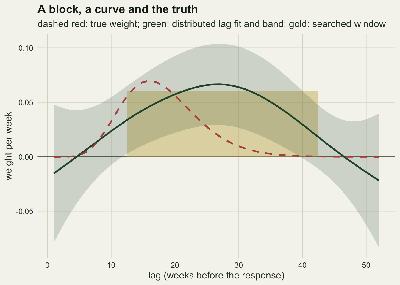
One dataset shows what the two answers look like, not how often either is right. That needs replicates.
The window’s slope is two errors pulling opposite ways
Five settings are simulated, 200 datasets each, with the number of replicates fixed before running and each coverage printed with its Monte Carlo standard error. Four use the narrow hump: independent weeks at 30 years, autocorrelated weeks at 30 and 60 years, all with an R-squared of 0.25, and independent weeks at 30 years with an R-squared of 0.5. The fifth uses the broad hump with autocorrelated weeks at 30 years. Each dataset gets the full search and one distributed lag fit; the second setting also gets fits with k = 6 and k = 15 on the same data.
one_rep <- function(n_yr, phi, w_true, cor_mat, sig, k_extra = NULL) {
  clim <- sim_clim(n_yr, phi)
  y    <- drop(clim %*% w_true) + rnorm(n_yr, 0, sig)
  rs   <- rect_search(clim, y)
  dl   <- lag_fit(clim, y)
  z95  <- qnorm(0.975)
  out <- c(rect     = rs$slope,
           rect_cov = rs$ci[1] <= 1 & rs$ci[2] >= 1,
           share    = sum(w_true[rs$open:rs$close]),
           pop      = pop_slope(rs$open, rs$close, w_true, cor_mat),
           r2_sel   = rs$r2,
           centre   = (rs$open + rs$close) / 2,
           width    = rs$close - rs$open + 1,
           dlm      = dl$total,
           dlm_cov  = abs(dl$total - 1) <= z95 * dl$total_se,
           dlm_se   = dl$total_se,
           peak     = lag_wk[which.max(dl$weight)],
           edf      = dl$edf)
  for (k in k_extra) {
    dk <- lag_fit(clim, y, k)
    out[paste0("cov_k", k)]  <- abs(dk$total - 1) <= z95 * dk$total_se
    out[paste0("peak_k", k)] <- lag_wk[which.max(dk$weight)]
  }
  out
}

scen <- data.frame(
  label = c("iid, R2 0.25, 30 yr", "AR 0.5, R2 0.25, 30 yr", "AR 0.5, R2 0.25, 60 yr",
            "iid, R2 0.5, 30 yr", "AR 0.5, broad, 30 yr"),
  phi   = c(0, 0.5, 0.5, 0, 0.5),
  r2    = c(0.25, 0.25, 0.25, 0.5, 0.25),
  n_yr  = c(30, 30, 60, 30, 30),
  hump  = c("narrow", "narrow", "narrow", "narrow", "broad"))
n_rep <- 200

set.seed(3102)
sim_out <- lapply(seq_len(nrow(scen)), function(i) {
  w_true  <- if (scen$hump[i] == "narrow") w_narrow else w_broad
  cor_mat <- ar_cor(scen$phi[i])
  sig     <- noise_sd(w_true, scen$phi[i], scen$r2[i])
  k_extra <- if (i == 2) c(6, 15) else NULL
  t(replicate(n_rep, one_rep(scen$n_yr[i], scen$phi[i], w_true, cor_mat, sig, k_extra)))
})

summ <- do.call(rbind, lapply(seq_along(sim_out), function(i) {
  m_i   <- sim_out[[i]]
  pk    <- if (scen$hump[i] == "narrow") peak_narrow else peak_broad
  infl  <- m_i[, "rect"] - m_i[, "pop"]
  miss  <- 1 - m_i[, "pop"]
  data.frame(label = scen$label[i],
             share = median(m_i[, "share"]), pop = median(m_i[, "pop"]),
             rect = median(m_i[, "rect"]), rect_q1 = quantile(m_i[, "rect"], 0.25),
             rect_q3 = quantile(m_i[, "rect"], 0.75), rect_mean = mean(m_i[, "rect"]),
             rect_cov = mean(m_i[, "rect_cov"]), width = median(m_i[, "width"]), r2_sel = median(m_i[, "r2_sel"]),
             infl = median(infl), miss = median(miss), miss_infl_cor = cor(miss, infl),
             dlm = median(m_i[, "dlm"]), dlm_q1 = quantile(m_i[, "dlm"], 0.25),
             dlm_q3 = quantile(m_i[, "dlm"], 0.75), dlm_mean = mean(m_i[, "dlm"]),
             dlm_cov = mean(m_i[, "dlm_cov"]),
             rect_sd = sd(m_i[, "rect"]), dlm_sd = sd(m_i[, "dlm"]),
             peak3 = mean(abs(m_i[, "peak"] - pk) <= 3),
             centre3 = mean(abs(m_i[, "centre"] - pk) <= 3),
             linear = mean(m_i[, "edf"] < 2.05),
             edge = mean(m_i[, "peak"] %in% c(1, n_lag)),
             row.names = NULL)
}))
mcse <- function(p) sqrt(p * (1 - p) / n_rep)
s1 <- summ[1, ]; s2 <- summ[2, ]; s3 <- summ[3, ]; s4 <- summ[4, ]; s5 <- summ[5, ]
share_30 <- range(summ$share[c(1, 2, 5)])
rect_all <- range(summ$rect)
rect_mean_30 <- range(summ$rect_mean[c(1, 2, 5)])
cov_rect_30 <- range(summ$rect_cov[c(1, 2, 5)])
miss_cor <- range(summ$miss_infl_cor)
At 30 years with the narrow hump, the searched window holds a median share of 0.655 of the true weight with independent weeks and 0.649 with autocorrelated weeks. At 60 years the median share rises to 0.776. The search at 30 years does not recover the infinite-data rectangle of 16 weeks: its median width is 13.5 weeks with independent weeks and 12.5 with autocorrelated weeks, and in the median dataset about a third of the hump is left outside.
The median slope of the selected window tells a different story: 1.018 and 0.997 at 30 years, 0.979 at 60, against a true total of one. Across all five settings the median slope lies between 0.941 and 1.018. A reader who checks the point estimate against the truth would conclude that the window works.
It does not, and the decomposition says why. The slope a regression on the chosen window would give with unlimited years is its population slope, which in the autocorrelated setting at 30 years has a median of 0.710. That is a median missing weight of 0.290. The median gap between the fitted slope and the population slope is 0.329: the search picked the window whose noise happened to line up with the response, and the slope carries that luck. So the window is missing weight in one direction and inflated by selection in the other, and in the middle of the distribution the two are of similar size. They do not offset each other dataset by dataset. The correlation between the missing weight and the inflation across datasets is negative in every setting, from -0.54 to -0.20: a window that misses more weight is, if anything, less inflated, so its slope tends to fall further below the truth rather than being pulled back towards it. That correlation describes single datasets; it says nothing about why the two medians agree. Both terms shrink as the record lengthens or the signal strengthens, and the median balance held in all five settings here. Nothing in this simulation explains it, and it is a property of the medians only. The means show the imbalance the medians hide: at 30 years the mean slope is between 0.872 and 0.936.
I expected the balance to break down at the stronger signal. With independent weeks and an R-squared of 0.5 the median share is 0.808, the median inflation 0.186 (against 0.344 at an R-squared of 0.25), and the median slope 0.952. Selection inflates less when the signal is strong, as the checking companion found, but the window also misses less weight, so the median slope still sits near one. The balance held through that change too, which makes a slope near one more reassuring than it deserves, not less. What it does not rescue is the interval.
The interval is where the window fails
cov_tab <- rbind(
  data.frame(label = scen$label, method = "searched window", cover = summ$rect_cov),
  data.frame(label = scen$label, method = "distributed lag", cover = summ$dlm_cov))
cov_tab$se    <- mcse(cov_tab$cover)
cov_tab$label <- factor(cov_tab$label, levels = rev(scen$label))
dlm_cov_rng   <- range(summ$dlm_cov)
dlm_med_rng   <- range(summ$dlm)
dlm_z_max     <- max(abs(summ$dlm_cov - 0.95) / mcse(summ$dlm_cov))
se_ratio_2    <- s2$dlm_sd / s2$rect_sd
se_ratio_3    <- s3$dlm_sd / s3$rect_sd
cov_k6  <- mean(sim_out[[2]][, "cov_k6"])
cov_k15 <- mean(sim_out[[2]][, "cov_k15"])
The naive 95 per cent interval on the selected window’s slope covers the true total of one in 0.665 of datasets with independent weeks and 0.600 with autocorrelated weeks at 30 years (Monte Carlo standard errors 0.033 and 0.035). At 60 years it covers in 0.785, and in the R-squared 0.5 setting in 0.735. The coverage falls short of 0.95 in every setting because the interval is centred on a slope that both misses part of the weight and carries the selection luck described above, and its width accounts for neither.
The distributed lag model’s total has a median between 0.955 and 1.037 across the five settings. Its interval is the Bayesian credible interval that mgcv’s vcov supplies by default, the posterior covariance of the coefficients given the smoothing parameter, which Marra and Wood showed has close to nominal frequentist coverage when averaged across the function; here it is applied to a sum over the whole function, a use their result does not directly cover, which is why it is measured. Over the five settings it covers the true total in between 0.915 and 0.965 of datasets, with a Monte Carlo standard error near 0.019; the setting furthest from 0.95 is 1.8 standard errors away. In the autocorrelated setting at 30 years it covers in 0.915.
That coverage is not bought with precision. In the autocorrelated setting at 30 years the standard deviation of the distributed lag total across datasets is 0.620 against 0.648 for the window slope, a ratio of 0.96; at 60 years the ratio is 1.14. Both estimators are noisy with thirty years of data. The difference is that one of them says so.
The basis size does not move this. Refitting the same 200 autocorrelated datasets at 30 years with k = 6 and k = 15 gives coverages of 0.915 and 0.915, against 0.915 with k = 10.
p_cov <- ggplot(cov_tab, aes(cover, label, colour = method)) +
  geom_vline(xintercept = 0.95, linetype = "dashed", colour = te_body, linewidth = 0.5) +
  geom_errorbar(aes(xmin = cover - 2 * se, xmax = cover + 2 * se), orientation = "y",
                width = 0.25, linewidth = 0.6, position = position_dodge(width = 0.5)) +
  geom_point(size = 2.4, position = position_dodge(width = 0.5)) +
  scale_colour_manual(values = c("distributed lag" = te_forest, "searched window" = te_rust),
                      name = NULL) +
  scale_x_continuous(limits = c(0.4, 1)) +
  labs(x = "coverage of the true total", y = NULL, title = "Interval coverage") +
  guides(colour = guide_legend(nrow = 2)) +
  theme_datasheet() +
  theme(legend.position = "bottom")

est_tab <- rbind(
  data.frame(label = scen$label, what = "window slope", mid = summ$rect,
             lo = summ$rect_q1, hi = summ$rect_q3),
  data.frame(label = scen$label, what = "distributed lag total", mid = summ$dlm,
             lo = summ$dlm_q1, hi = summ$dlm_q3),
  data.frame(label = scen$label, what = "share in window", mid = summ$share,
             lo = summ$share, hi = summ$share))
est_tab$label <- factor(est_tab$label, levels = rev(scen$label))

p_est <- ggplot(est_tab, aes(mid, label, colour = what)) +
  geom_vline(xintercept = 1, linetype = "dashed", colour = te_body, linewidth = 0.5) +
  geom_errorbar(aes(xmin = lo, xmax = hi), orientation = "y", width = 0.25,
                linewidth = 0.6, position = position_dodge(width = 0.6)) +
  geom_point(size = 2.4, position = position_dodge(width = 0.6)) +
  scale_colour_manual(values = c("distributed lag total" = te_forest,
                                 "window slope" = te_rust, "share in window" = te_gold),
                      name = NULL) +
  labs(x = "estimate (true total = 1)", y = NULL, title = "Medians and quartiles") +
  theme_datasheet() +
  guides(colour = guide_legend(nrow = 2)) +
  theme(legend.position = "bottom", axis.text.y = element_blank())

p_cov + p_est + plot_annotation(theme = theme_datasheet())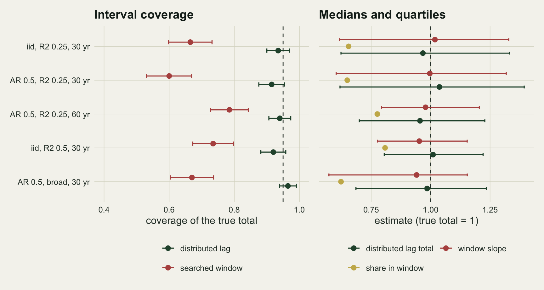
Where the effect sits is the harder question
peak_long <- do.call(rbind, lapply(1:4, function(i) {
  data.frame(label = scen$label[i], peak = sim_out[[i]][, "peak"])
}))
peak_long$label <- factor(peak_long$label, levels = scen$label[1:4])
peak3_k6  <- mean(abs(sim_out[[2]][, "peak_k6"] - peak_narrow) <= 3)
peak3_k15 <- mean(abs(sim_out[[2]][, "peak_k15"] - peak_narrow) <= 3)
lin_edge_2 <- mean(sim_out[[2]][sim_out[[2]][, "edf"] < 2.05, "peak"] %in% c(1, n_lag))
The distributed lag model knows the total. It does not know where the effect sits. Counting a fitted peak as recovered when it lies within three weeks of the true peak at week 16, the model recovers it in 0.320 of datasets with independent weeks and 0.295 with autocorrelated weeks at 30 years (Monte Carlo standard errors near 0.032). At 60 years that rises to 0.640, and with the stronger signal at 30 years to 0.755. For the broad hump at 30 years it is 0.305.
The reason is visible in the effective degrees of freedom. The penalty on the spline is on its second derivative, so a straight line in lag costs nothing, and with 30 noisy years REML often decides that a straight line is all the data support. In the autocorrelated setting at 30 years the weight curve used two effective degrees of freedom or fewer, a straight line, in 0.395 of datasets; the fraction of those straight-line fits with the peak at lag 1 or lag 52 is 1.000, as a straight line must. Overall the peak landed on one of the two end lags in 0.500 of datasets at 30 years and 0.215 at 60. A straight-line weight still sums to a sensible total, which is why the interval above is fine and the peak is not.
The searched window does better at this. Its centre lies within three weeks of the true peak in 0.540 of autocorrelated datasets at 30 years, against 0.295 for the distributed lag peak. That is not a point in the window’s favour as a method, because its interval is the one that fails, but it rules out selling the distributed lag model as the way to find the timing from thirty years. Changing the basis size does not help either: with k = 6 and k = 15 the peak is recovered in 0.270 and 0.295 of the same datasets.
ggplot(peak_long, aes(peak)) +
  annotate("rect", xmin = peak_narrow - 3.5, xmax = peak_narrow + 3.5, ymin = -Inf, ymax = Inf,
           fill = te_gold, alpha = 0.3) +
  geom_histogram(binwidth = 1, fill = te_forest, colour = NA) +
  facet_wrap(~ label, ncol = 2) +
  labs(x = "fitted peak lag (weeks)", y = "datasets",
       title = "The total is found; the timing often is not",
       subtitle = "gold band: true peak at week 16, plus or minus three weeks") +
  theme_datasheet()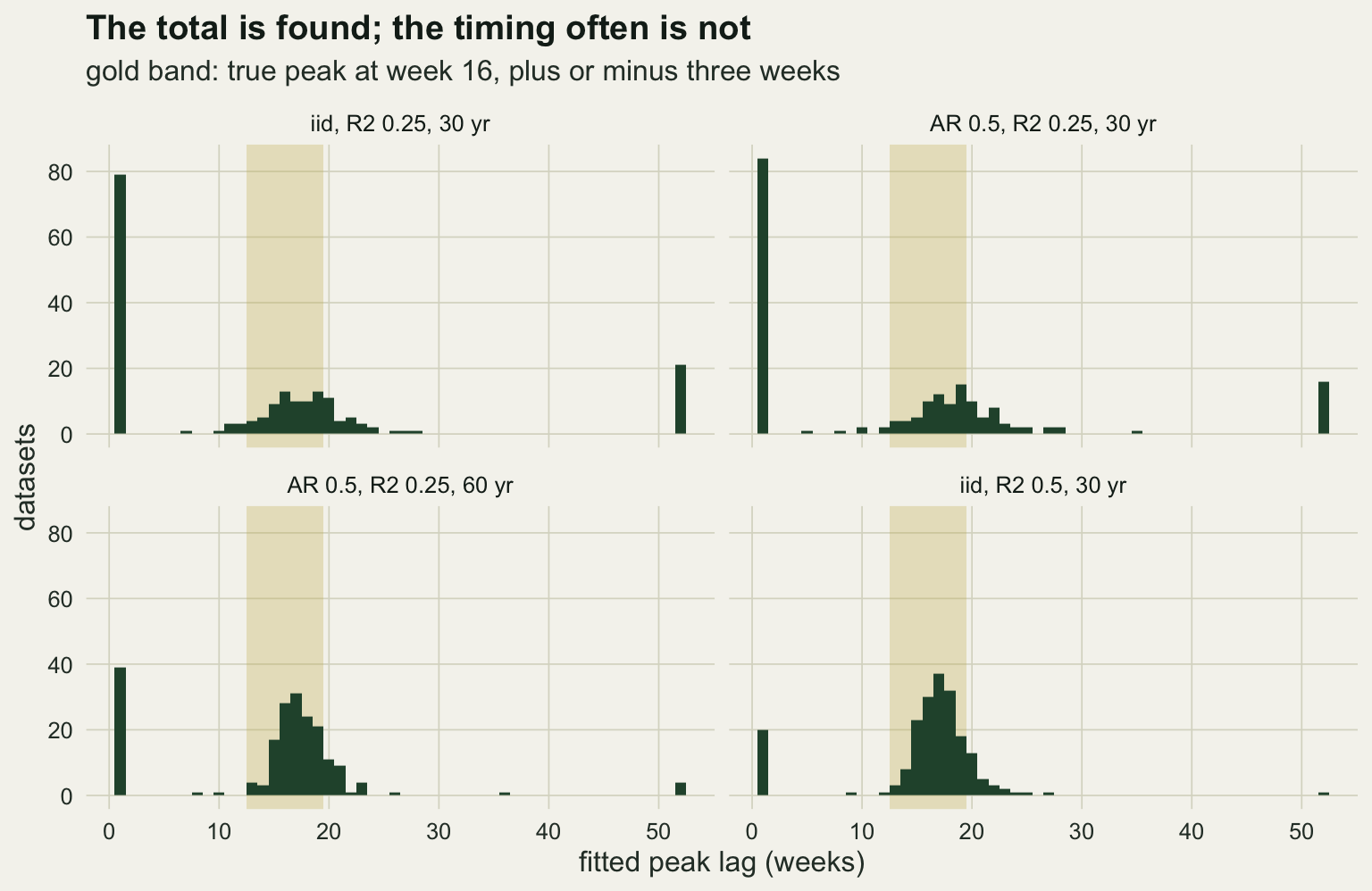
What to report
Report the total effect of a sustained anomaly with its interval, and fit it as a distributed lag rather than reading it off a searched window. In these simulations the window’s naive interval covered the truth in as few as 0.600 of datasets at 30 years, while the distributed lag interval was never more than 1.8 Monte Carlo standard errors from 0.95. Name the interval as a Bayesian credible interval from the penalised fit, since that is what vcov on a gam returns.
If a window has been searched, do not take comfort from a slope close to what theory expects. In these settings the median window slope was near the truth because two biases of opposite sign were similar in size at the median in every setting tried, and the window held only 0.623 to 0.655 of the weight at 30 years.
Report the fitted weight curve with its band and the effective degrees of freedom of the lag smooth. If that number is two, the model has fitted a straight line in lag and says nothing about timing; quote the total and say the timing was not resolved. Quote a peak lag only with a record long enough to support it, and check that length by simulating from a weight shaped like the one you believe.
Honest limits
Everything above is linear: the response is a weighted sum of weekly anomalies with no threshold, no interaction with a second variable, and Gaussian noise. The distributed lag non-linear models of Gasparrini and colleagues allow the effect to curve in the exposure as well as in lag, and a tensor product smooth in mgcv does the same; neither was fitted, and their coverage at 30 years is not measured here.
The true weight is a gamma density that is positive at every lag, and the fitted weight is unconstrained. A real lag weight that changes sign, such as warmth that helps in one season and harms in the next, would change both the share arithmetic and the straight-line collapse. Penalties whose null space excludes the straight line, or that shrink the weight towards zero at long lags, would probably change the peak-lag result; that was not tested. The coverage figure comes from 200 datasets per setting, so a true coverage within about 0.038 of each distributed lag coverage and about 0.069 of each window coverage is compatible with the simulation.
The search is the simplest version: every contiguous window, R-squared as the criterion, one climate variable, no randomisation null. Climate window analysis shows how a randomisation of the response repairs the false positive rate of such a search, and van de Pol and colleagues set out the sliding-window search this post imitates together with its randomisation checks; that null was not run here. A weighted window with a fitted kernel is closer in spirit to the distributed lag model than to the rectangle tested above, and was not tested either. Teller and colleagues fitted climate effects on demographic rates as smooth functions of lagged covariates in the same linear functional form, which is the ecological precedent for the model used here.
My expectation that the window slope would clearly undershoot at an R-squared of 0.5 did not hold in this measurement: the median slope stayed near one. Whether the two biases stay in balance for a narrower hump, a much longer search grid or a different selection criterion is open.
References
Gasparrini A, Armstrong B, Kenward MG 2010 Statistics in Medicine 29(21):2224-2234 (10.1002/sim.3940)
van de Pol M, Bailey LD, McLean N, Rijsdijk L, Lawson CR, Brouwer L 2016 Methods in Ecology and Evolution 7(10):1246-1257 (10.1111/2041-210X.12590)
Teller BJ, Adler PB, Edwards CB, Hooker G, Ellner SP 2016 Methods in Ecology and Evolution 7(2):171-183 (10.1111/2041-210X.12486)
Wood SN 2011 Journal of the Royal Statistical Society Series B 73(1):3-36 (10.1111/j.1467-9868.2010.00749.x)
Marra G, Wood SN 2012 Scandinavian Journal of Statistics 39(1):53-74 (10.1111/j.1467-9469.2011.00760.x)