---
title: "Jensen's inequality and thermal variability"
description: "Jensen's inequality on a thermal performance curve: fluctuating-temperature performance is not performance at the mean, and the best mean is below the optimum."
date: "2026-06-29 15:00"
date-modified: "2026-10-14"
categories: [ecology tutorial, R, thermal ecology, climate change, physiology]
image: thumbnail.png
image-alt: "A thermal performance curve with a temperature distribution near the optimum, showing mean performance falling below the performance at the mean temperature."
---
*Corrected 14 October 2026: the post said the best mean temperature sits far enough down the rising limb that a warm excursion cannot fling the organism over the cliff; under the Normal temperature distribution the post uses, warm excursions still do so at the best mean, and the text now says they do so less often there than at the optimum, at the price of a little performance at the mean.*
*Corrected 7 October 2026: the post said the best mean temperature sits below the optimum because variability near the peak costs performance; it now says this also needs the curve to be asymmetric, and that the inflection marks the boundary between variability helping and hurting only when the variability is small.*
```{r setup}
#| code-fold: true
#| code-summary: "Setup: packages, colours and plot theme"
#| results: hide
#| message: false
#| warning: false
knitr::opts_chunk$set(echo = TRUE, message = FALSE, warning = FALSE,
                      dev = "png", dpi = 120, fig.path = "figures/",
                      fig.width = 7, fig.height = 4.4)
library(ggplot2)
theme_te <- theme_minimal(base_size = 12) +
  theme(panel.background = element_rect(fill = "#f5f4ee", colour = NA),
        plot.background  = element_rect(fill = "#f5f4ee", colour = NA),
        panel.grid.minor = element_blank(),
        plot.title = element_text(face = "bold", size = 12))
theme_set(theme_te)
col_curve <- "#3a6b52"; col_hi <- "#b5651d"; col_ref <- "#555555"

briere <- function(T, a = 8e-4, T0 = 8, Tm = 42) {
  p <- a*T*(T-T0)*sqrt(pmax(Tm-T, 0)); p[T < T0 | T > Tm] <- 0; p }
Tg <- seq(0, 45, 0.005); Pg <- briere(Tg); Topt <- Tg[which.max(Pg)]

## inflection on the rising limb (curvature sign change)
d2 <- diff(Pg, differences = 2)
infl_all <- Tg[which(diff(sign(d2)) != 0) + 1]
infl <- infl_all[infl_all > 12 & infl_all < Topt][1]

## expected performance over Normal(mu, sd)
EP <- function(mu, sd) { x <- seq(mu-4*sd, mu+4*sd, length = 4001); w <- dnorm(x, mu, sd); sum(briere(x)*w)/sum(w) }

g_lo <- EP(20, 6) - briere(20)      # below inflection: helps
g_opt <- EP(Topt, 6) - briere(Topt) # at optimum: hurts
loss_opt <- 100 * (1 - EP(Topt, 6) / briere(Topt))

## loss at optimum vs sd
sds <- c(2, 4, 6, 8)
loss_tab <- sapply(sds, function(s) 100 * (1 - EP(Topt, s) / briere(Topt)))

## optimal mean temperature vs sd
best_mu <- function(sd) { mus <- seq(20, 40, 0.05); mus[which.max(sapply(mus, EP, sd = sd))] }
bm <- sapply(c(3, 6, 9), best_mu); shift <- Topt - bm
```
An organism almost never experiences its mean temperature. It experiences a distribution: warm afternoons, cool nights, a hot week, a cold snap. If the thermal performance curve were a straight line this would not matter, because the average of a linear function is the function of the average. But the [performance curve is not a line](../thermal-performance-curves/); it bends, and once a function bends, the average performance and the performance at the average part company. That gap is Jensen's inequality, and in thermal ecology it has real teeth (Martin and Huey 2008 The American Naturalist 171(3):E102-E118).
## The fallacy of the average
Jensen's inequality says that for a concave (bending downward) function, the average of the outputs is *less* than the output at the average input; for a convex (bending upward) function it is *more*. A performance curve is concave near its peak and convex on its accelerating lower limb, so thermal variability does opposite things depending on where the organism sits.
Compute expected performance directly, by averaging the curve over a temperature distribution.
```{r ep}
briere <- function(T, a = 8e-4, T0 = 8, Tm = 42) {
  p <- a*T*(T-T0)*sqrt(pmax(Tm-T, 0)); p[T < T0 | T > Tm] <- 0; p }
EP <- function(mu, sd) {                       # expected performance over Normal(mu, sd)
  x <- seq(mu-4*sd, mu+4*sd, length = 4001); w <- dnorm(x, mu, sd)
  sum(briere(x) * w) / sum(w)
}
c(at_mean_20  = briere(20),  expected_20  = EP(20, 6),
  at_mean_opt = briere(Topt), expected_opt = EP(Topt, 6))
```
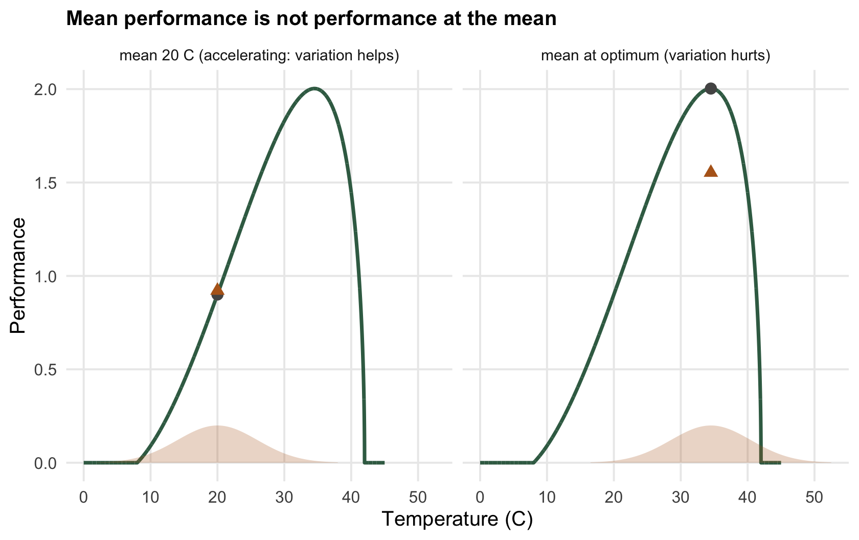
At a cool mean of 20 degrees C, on the accelerating part of the curve, adding a standard deviation of 6 degrees *raises* expected performance by `r sprintf("%.3f", g_lo)`: the warm excursions gain more than the cool ones lose. At the optimum the sign flips. The same variability *lowers* expected performance by `r sprintf("%.3f", -g_opt)`, a drop of `r sprintf("%.1f", loss_opt)` per cent, because every excursion, warm or cool, moves the organism off its peak, and the steep upper side punishes the warm ones hard. The curve changes from convex to concave near `r sprintf("%.0f", infl)` degrees; for small variability that inflection is the boundary between variability helping and hurting, and a wider spread moves the boundary a little cooler.
```{r fig-jensen}
#| fig-cap: "The same thermal variation at two mean temperatures. On the accelerating lower limb (left) averaging over the spread lifts performance above the value at the mean; near the optimum (right) it drops it below."
#| fig-alt: "Two panels of the performance curve, each with a bell-shaped temperature distribution; on the left the expected performance is above the point at the mean, on the right it is below."
mk <- function(mu, sd = 6, lab) {
  xs <- seq(mu-3*sd, mu+3*sd, 0.1)
  data.frame(T = xs, dens = dnorm(xs, mu, sd), mu = mu, lab = lab,
             at = briere(mu), ex = EP(mu, sd))
}
band <- rbind(mk(20, lab = "mean 20 C (accelerating: variation helps)"),
              mk(Topt, lab = "mean at optimum (variation hurts)"))
cur  <- data.frame(T = Tg, P = Pg)
ggplot() +
  geom_line(data = cur, aes(T, P), colour = col_curve, linewidth = 1) +
  geom_area(data = band, aes(T, dens * 3), fill = col_hi, alpha = 0.25) +
  geom_point(data = unique(band[, c("mu","at","lab")]), aes(mu, at), colour = col_ref, size = 2.6) +
  geom_point(data = unique(band[, c("mu","ex","lab")]), aes(mu, ex), colour = col_hi, size = 2.6, shape = 17) +
  facet_wrap(~lab) +
  labs(x = "Temperature (C)", y = "Performance",
       title = "Mean performance is not performance at the mean") +
  theme(strip.text = element_text(size = 9))
```
The grey circle is performance at the mean temperature; the ochre triangle is the true expected performance once you average over the spread. On the left the triangle sits above the circle, on the right below.
## Why the best mean is below the optimum
This has a striking consequence. Because variability near the peak costs performance and the curve is asymmetric, steeper above the optimum than below it, the best mean temperature to experience is not the optimum itself: it is somewhere cooler, far enough down the gentle rising limb that warm excursions fling the organism over the cliff less often, at the price of a little performance at the mean. Find the mean that maximises expected performance.
```{r best-mean}
best_mu <- function(sd) { mus <- seq(20, 40, 0.05); mus[which.max(sapply(mus, EP, sd = sd))] }
sapply(c(3, 6, 9), best_mu)          # optimal mean temperature at three variability levels
```
With a thermal standard deviation of 3 degrees the best mean sits `r sprintf("%.1f", shift[1])` degrees below the optimum; at 6 degrees, `r sprintf("%.1f", shift[2])` below; at 9 degrees, `r sprintf("%.1f", shift[3])` below. This is why "suboptimal is optimal": a lizard that thermoregulates to a body temperature a few degrees under its measured performance peak is not making a mistake, it is buying insurance against the steep side of its own curve (Martin and Huey 2008).
```{r fig-loss}
#| fig-cap: "Performance loss at the optimum grows with thermal variability. Averaging a concave peak over a wider spread costs more, so a more variable climate erodes performance even with no change in the mean."
#| fig-alt: "A rising curve showing per cent performance loss at the optimum against thermal standard deviation, from zero with no variability to about a third at high variability."
dl <- data.frame(sd = seq(0, 9, 0.25))
dl$loss <- sapply(dl$sd, function(s) if (s == 0) 0 else 100 * (1 - EP(Topt, s) / briere(Topt)))
ggplot(dl, aes(sd, loss)) +
  geom_line(colour = col_hi, linewidth = 1) +
  labs(x = "Thermal standard deviation (C)", y = "Performance loss at the optimum (%)",
       title = "More variable, not warmer: variance alone costs performance")
```
## The honest limits
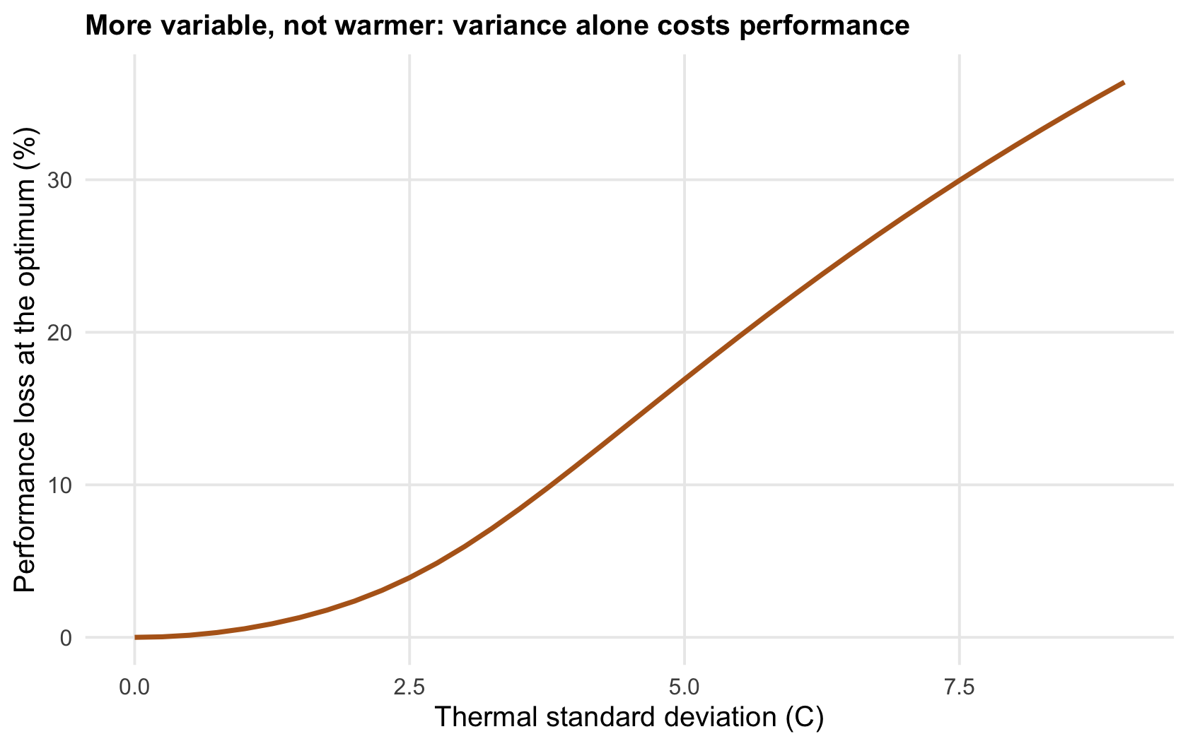
Two caveats keep this from being a universal law. First, it assumes the organism takes the temperature it is given. Behavioural thermoregulation, moving into shade, basking, shifting activity to dawn, lets many ectotherms edit their own temperature distribution, and a good deal of ecology is exactly that editing. Second, it assumes the curve measured under constant conditions applies instant by instant. Real physiology has memory: acclimation and thermal history shift the curve, so rapid fluctuations and slow seasonal change are not the same thing (Sinclair et al. 2016 Ecology Letters 19(11):1372-1385). Even with those caveats, the direction holds and it matters for climate: a rise in thermal *variance* can erode performance on its own, without any change in the mean (Vasseur et al. 2014 Proceedings of the Royal Society B 281(1779):20132612). The next post turns the mean back on and asks which species warming actually threatens.
## References
- Martin TL, Huey RB 2008. The American Naturalist 171(3):E102-E118 (10.1086/527502).
- Sinclair BJ et al. 2016. Ecology Letters 19(11):1372-1385 (10.1111/ele.12686).
- Vasseur DA et al. 2014. Proceedings of the Royal Society B 281(1779):20132612 (10.1098/rspb.2013.2612).
## Related tutorials
- [Thermal performance curves in R](../thermal-performance-curves/)
- [Thermal safety margins and warming](../thermal-safety-margins-and-warming/)
- [Checking a thermal performance analysis](../checking-a-thermal-performance-analysis/)
- [Leaf area from gap fraction: the segment length](../leaf-area-from-gap-fraction/)