library(ggplot2)
library(patchwork)

te_paper  <- "#f5f4ee"
te_ink    <- "#16241d"
te_body   <- "#2c3a31"
te_forest <- "#275139"
te_rust   <- "#b5534e"
te_gold   <- "#c9b458"
te_line   <- "#dad9ca"

theme_datasheet <- function() {
  theme_minimal(base_size = 12) +
    theme(plot.background  = element_rect(fill = te_paper, colour = NA),
          panel.background = element_rect(fill = te_paper, colour = NA),
          panel.grid.major = element_line(colour = te_line, linewidth = 0.3),
          panel.grid.minor = element_blank(),
          text             = element_text(colour = te_body),
          plot.title       = element_text(colour = te_ink, face = "bold"),
          plot.subtitle    = element_text(colour = te_body),
          axis.text        = element_text(colour = te_body),
          strip.text       = element_text(colour = te_ink))
}Leaf area from gap fraction: the segment length
R
leaf area index
canopy
remote sensing
simulation
ecology tutorial
Inverting canopy gap fraction to leaf area index in R: why long segments underestimate a clumped canopy, and why short ones saturate. Choosing segment length.
A forest plot is walked with an optical sensor, or photographed upward with a fisheye lens, and every reading is a gap fraction: the share of sky visible through the canopy along some line of sight. Leaf area index comes out of it through the Beer-Lambert law. If leaves are scattered at random, the probability that a beam at zenith angle theta passes through a layer of leaf area L without touching a leaf is exp(-G L / cos theta), where G is the projection of unit leaf area in the beam direction, so L is minus the log of the gap fraction, times cos theta, divided by G. The simulation in this post uses a vertical beam, so cos theta is 1 and the formula reduces to exp(-G L). The algebra is one line and every canopy instrument does it.
The trouble is that canopies are not random. Leaves sit in crowns and crowns sit in clumps with holes between them. A beam through a dense crown and a beam through a gap between crowns are averaged into one gap fraction, and the log of that average is not the average of the logs. Nilson set this out in 1971; Lang and Xiang proposed in 1986 to take the log over short segments of a transect first and average the logged values afterwards, so that each segment sees a roughly homogeneous piece of canopy. The practical question that proposal leaves open is how short a segment should be, and that is the question this post measures.
The same patchiness has already appeared on this site as a variance problem. Estimating plant cover with point intercepts shows that a hundred pins in a frame over patchy vegetation are not a hundred independent samples, but the cover estimate there is a proportion and stays unbiased; nothing is logged. Here the patchiness passes through a log and becomes a bias. The general inequality behind that bias is the subject of Jensen’s inequality and thermal variability, which works on a performance curve and has no finite sample and no zero reading to worry about. Gap fraction has both, and the second is where short segments go wrong: a segment with no gap at all has an infinite logged value and has to be floored or thrown away. A closed canopy that stops letting signal through is also the failure met in LiDAR height normalisation on slopes, where the ground returns run out.
The post does three things. It writes the long-segment bias in closed form for a gamma-distributed canopy and checks the simulation against it. It then sweeps segment length along simulated transects with three clump sizes and three degrees of clumping, and measures where the log-average comes closest to the truth and why. Finally it compares the two ways of handling saturated segments.
The log of a mean gap fraction has a closed-form bias
Take a canopy in which the leaf area along a beam varies from place to place, and within one place leaves are random. The gap fraction averaged over many places is the mean of exp(-G L). If L follows a gamma distribution with mean Lbar and coefficient of variation cv, that mean is the gamma moment generating function evaluated at -G, which is (1 + G Lbar cv^2) raised to the power -1/cv^2. Logging it and dividing by G gives what an instrument reports from one long average, often called effective leaf area index. Its ratio to the true mean is log(1 + G Lbar cv^2) divided by cv^2 G Lbar. The ratio depends on the product G Lbar, so denser canopies lose more, and it goes to one as cv goes to zero.
The design constants below were fixed before any simulation ran: G of 0.5, which is the value for a spherical leaf angle distribution (and very nearly the value for any leaf angle distribution at a zenith angle of 57.5 degrees, although the beam simulated here is vertical and only the value of G is borrowed); a mean leaf area index of 3; transects of 1920 beams; and 800 transects per cell.
g_proj  <- 0.5
lai_bar <- 3
n_beam  <- 1920
n_tr    <- 800

eff_ratio <- function(cv) ifelse(cv == 0, 1,
  log(1 + g_proj * lai_bar * cv^2) / (cv^2 * g_proj * lai_bar))

cf_half <- eff_ratio(0.5)
cf_one  <- eff_ratio(1)
For a moderately clumped canopy with a coefficient of variation of 0.5 the long average recovers 0.849 of the true leaf area; at a coefficient of variation of 1 it recovers 0.611. Nothing here is estimated. The number is fixed by G, the mean and the clumping.
The simulator that the rest of the post uses builds a transect from patches of constant leaf area, each patch a run of beams whose leaf area is a gamma draw, with the patch boundaries placed at a random offset so that they do not line up with the segments. Every beam is a Bernoulli gap with probability exp(-G L). The truth for each transect is its own realised mean leaf area, so the sampling variation of the canopy is removed from the comparison.
seg_grid   <- c(4, 8, 10, 16, 24, 32, 40, 60, 96, 160, 240, 480, 1920)
cv_grid    <- c(0, 0.5, 1)
patch_grid <- c(10, 40, 160)

make_transects <- function(cv, patch, offset_random = TRUE) {
  n_patch <- ceiling(n_beam / patch) + 1
  lai_patch <- if (cv == 0) matrix(lai_bar, n_tr, n_patch) else
    matrix(rgamma(n_tr * n_patch, shape = 1 / cv^2, scale = lai_bar * cv^2),
           n_tr, n_patch)
  offset <- if (offset_random) sample.int(patch, n_tr, replace = TRUE) - 1 else
    rep(0, n_tr)
  patch_id <- outer(offset, seq_len(n_beam) - 1, "+") %/% patch + 1
  lai_beam <- matrix(lai_patch[cbind(rep(seq_len(n_tr), n_beam),
                                     as.vector(patch_id))], n_tr, n_beam)
  gap <- matrix(rbinom(n_tr * n_beam, 1, exp(-g_proj * lai_beam)), n_tr, n_beam)
  list(gap = gap, truth = rowMeans(lai_beam))
}

rel_floor_of <- function(tr, m) {
  counts <- t(rowsum(t(tr$gap), rep(seq_len(n_beam / m), each = m)))
  rowMeans(-log(pmax(counts / m, 1 / (2 * m)))) / g_proj / tr$truth
}

estimate_segments <- function(tr, m) {
  n_seg <- n_beam / m
  seg_id <- rep(seq_len(n_seg), each = m)
  counts <- t(rowsum(t(tr$gap), seg_id))
  frac   <- counts / m
  lx_floor <- rowMeans(-log(pmax(frac, 1 / (2 * m)))) / g_proj
  log_frac <- ifelse(frac > 0, -log(pmax(frac, 1e-300)), NA)
  lx_drop  <- rowMeans(log_frac, na.rm = TRUE) / g_proj
  rel_floor <- lx_floor / tr$truth
  rel_drop  <- lx_drop / tr$truth
  c(m = m,
    floor = mean(rel_floor), floor_se = sd(rel_floor) / sqrt(n_tr),
    floor_rmse = sqrt(mean((rel_floor - 1)^2)),
    drop = mean(rel_drop, na.rm = TRUE),
    saturated = mean(counts == 0))
}set.seed(6211)
cell_list <- list()
rel_store <- list()
for (patch in patch_grid) for (cv in cv_grid) {
tr <- make_transects(cv, patch)
est <- t(vapply(seg_grid, function(m) estimate_segments(tr, m), numeric(6)))
cell_list[[length(cell_list) + 1]] <- data.frame(cv = cv, patch = patch, est)
if (cv == 1) rel_store[[as.character(patch)]] <-
vapply(seg_grid, function(m) rel_floor_of(tr, m), numeric(n_tr))
}
sweep_tab <- do.call(rbind, cell_list)
long_rows <- sweep_tab[sweep_tab$m == n_beam, ]
sim_long <- function(cv, patch) long_rows$floor[long_rows$cv == cv & long_rows$patch == patch]
se_long <- function(cv, patch) long_rows$floor_se[long_rows$cv == cv & long_rows$patch == patch]
gap_half <- sim_long(0.5, 10) - cf_half
gap_one <- sim_long(1, 10) - cf_one
gap_one_160 <- sim_long(1, 160) - cf_oneWith one segment covering the whole transect the Lang-Xiang average and the log of the mean gap fraction are the same number, so the last column of the sweep is the closed form’s test. The formula is the limit of many patches and many beams. A finite transect sits slightly above it for two reasons that both push upwards: the log of a sample mean over a limited number of patches is itself a biased estimate of the log of the population mean, and the gap fraction is a binomial proportion out of 1920 beams, whose minus-log is convex. With patches of 10 beams, which gives each transect about 192 independent patches, the simulated ratio is 0.852 against the closed-form 0.849 at a coefficient of variation of 0.5 (difference +0.003, Monte Carlo standard error 0.001), and 0.612 against 0.611 at 1 (difference +0.001, standard error 0.001). With patches of 160 beams each transect holds only 12 patches, and the simulated ratio at a coefficient of variation of 1 rises to 0.643, +0.032 from the formula, because with a dozen crowns per transect the first of those two terms is no longer small.
cf_curve <- data.frame(cv = seq(0, 1.5, by = 0.01))
cf_curve$ratio <- eff_ratio(cf_curve$cv)
long_pts <- long_rows[long_rows$cv > 0, ]
long_pts$patch_lab <- factor(paste(long_pts$patch, "beam patches"),
                             levels = paste(patch_grid, "beam patches"))

ggplot(cf_curve, aes(cv, ratio)) +
  geom_hline(yintercept = 1, linetype = "dashed", colour = te_body, linewidth = 0.5) +
  geom_line(colour = te_forest, linewidth = 1) +
  geom_point(data = long_pts, aes(cv, floor, colour = patch_lab), size = 2.6,
             position = position_dodge(width = 0.06)) +
  scale_colour_manual(values = c(te_gold, te_rust, te_ink), name = NULL) +
  scale_y_continuous(limits = c(0.4, 1.02)) +
  labs(x = "coefficient of variation of patch leaf area",
       y = "estimated / true leaf area index",
       title = "Averaging before the log loses leaf area",
       subtitle = "green line: closed form; points: one segment per 1920-beam transect") +
  theme_datasheet() +
  theme(legend.position = "bottom")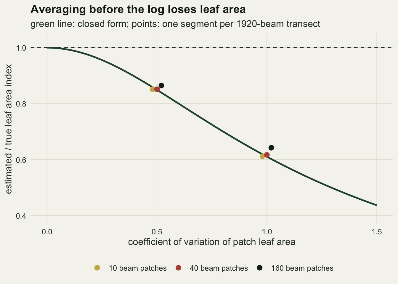
Shorter segments bring two new errors
Cutting the transect into segments of m beams and averaging the logged segment values removes the between-patch part of the Jensen gap, but each segment gap fraction is now a proportion out of m Bernoulli trials. Two things follow. Minus the log is convex, so even in a perfectly random canopy the expected log of a noisy proportion sits above the log of the true proportion, and short segments overestimate. And a segment in which no beam gets through has no finite log at all. The rule used first here replaces a zero count by half a beam, a floor of 1/(2m), which caps the leaf area a single segment can report at log(2m)/G.
For an unclumped canopy both effects can be computed exactly by summing over the binomial distribution of the gap count, which gives a second check on the simulator.
exact_floor <- function(m) {
  k_vals <- 0:m
  p_gap  <- exp(-g_proj * lai_bar)
  sum(dbinom(k_vals, m, p_gap) * -log(pmax(k_vals / m, 1 / (2 * m)))) /
    (g_proj * lai_bar)
}
check_m   <- c(4, 8, 16, 40)
exact_vals <- vapply(check_m, exact_floor, 0)
sim_vals  <- sweep_tab$floor[sweep_tab$cv == 0 & sweep_tab$patch == 40 &
                             sweep_tab$m %in% check_m]
sim_ses   <- sweep_tab$floor_se[sweep_tab$cv == 0 & sweep_tab$patch == 40 &
                                sweep_tab$m %in% check_m]
check_z   <- max(abs(sim_vals - exact_vals) / sim_ses)
check_zm  <- check_m[which.max(abs(sim_vals - exact_vals) / sim_ses)]
check_abs <- max(abs(sim_vals - exact_vals))
sat_exact_4 <- (1 - exp(-g_proj * lai_bar))^4
cap_4     <- log(8) / g_proj
In a random canopy with a leaf area index of 3 the exact expectation of the floored estimator, relative to the truth, is 0.982 at 4-beam segments, 1.100 at 8, 1.086 at 16 and 1.032 at 40. The simulated values differ from these by at most 0.0028; the largest standardised discrepancy is 2.6 Monte Carlo standard errors, at 4 beams, which is larger than chance would usually give for four comparisons but small against every effect discussed below. The dip at 4 beams is the floor at work: a share of 0.364 of segments see no gap, and each is recorded at 4.16 in place of an infinite value, so the floor cuts off the whole upper tail of the logged proportion. From 8 beams onwards the convexity bias dominates; in the simulated sweep it is largest at 8 to 10 beams and shrinks as segments lengthen beyond that. So in a canopy with no clumping at all the log-average overestimates at intermediate segment lengths, and the bias fades only as the segments become long.
Clumping adds the Jensen gap back in, and it pulls the other way. The figure shows the floored Lang-Xiang estimate against segment length for every cell of the sweep.
best_tab <- do.call(rbind, lapply(split(sweep_tab, list(sweep_tab$cv, sweep_tab$patch)),
  function(d) d[which.min(abs(d$floor - 1)), ]))
best_tab <- best_tab[order(best_tab$cv, best_tab$patch), ]
best_of  <- function(cv, patch, col) best_tab[[col]][best_tab$cv == cv & best_tab$patch == patch]
at_patch <- function(cv, patch) sweep_tab$floor[sweep_tab$cv == cv & sweep_tab$patch == patch &
                                                sweep_tab$m == patch]
rmse_best <- do.call(rbind, lapply(split(sweep_tab, list(sweep_tab$cv, sweep_tab$patch)),
  function(d) d[which.min(d$floor_rmse), c("cv", "patch", "m", "floor_rmse")]))
max_se   <- max(sweep_tab$floor_se)

pair_tab <- do.call(rbind, lapply(patch_grid, function(pl) {
  rel  <- rel_store[[as.character(pl)]]
  bias <- abs(colMeans(rel) - 1)
  ord  <- order(bias)
  d    <- rel[, ord[1]] - rel[, ord[2]]
  data.frame(patch = pl, best_m = seg_grid[ord[1]], best = mean(rel[, ord[1]]),
             second_m = seg_grid[ord[2]], second = mean(rel[, ord[2]]),
             z = mean(d) / (sd(d) / sqrt(n_tr)))
}))
pair_of <- function(patch, col) pair_tab[[col]][pair_tab$patch == patch]
plot_sweep <- sweep_tab
plot_sweep$patch_lab <- factor(paste(plot_sweep$patch, "beam patches"),
levels = paste(patch_grid, "beam patches"))
plot_sweep$cv_lab <- factor(paste("cv", plot_sweep$cv))
patch_marks <- data.frame(patch_lab = factor(levels(plot_sweep$patch_lab),
levels = levels(plot_sweep$patch_lab)),
m = patch_grid)
ggplot(plot_sweep, aes(m, floor, colour = cv_lab)) +
geom_hline(yintercept = 1, linetype = "dashed", colour = te_body, linewidth = 0.5) +
geom_vline(data = patch_marks, aes(xintercept = m), linetype = "dotted",
colour = te_body, linewidth = 0.6) +
geom_line(linewidth = 0.9) +
geom_point(size = 1.8) +
facet_wrap(~ patch_lab, nrow = 1) +
scale_x_log10(breaks = c(4, 16, 60, 240, 1920)) +
scale_colour_manual(values = c(te_gold, te_forest, te_rust), name = NULL) +
labs(x = "segment length (beams, log scale)",
y = "estimated / true leaf area index",
title = "No segment length is right for every canopy",
subtitle = "floor rule; dashed: truth") +
theme_datasheet() +
theme(legend.position = "bottom")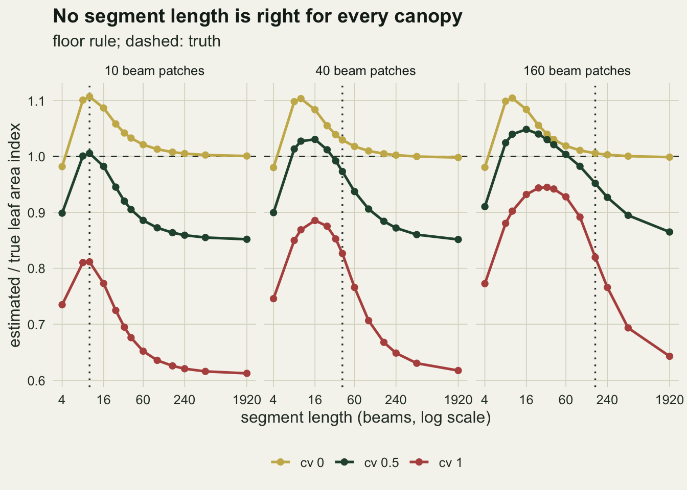
The largest Monte Carlo standard error of any point in the figure is 0.0045, so differences of a few hundredths are well outside the simulation noise. For the strongly clumped canopy (coefficient of variation 1) the log-average never reaches the truth. Its best value is 0.812 at 10-beam segments when patches are 10 beams long, 0.886 at 16 beams with 40-beam patches, and 0.945 at 32 beams with 160-beam patches. Setting the segment equal to the patch length does worse than that: 0.827 for 40-beam patches and 0.820 for 160-beam patches. The grid is fine enough near the peaks to compare neighbouring lengths on the same transects, and the paired differences separate one case from two ties. With 40-beam patches the best length, 16 beams, beats the runner-up at 24 beams (0.875) by a paired z of 18.7. With 160-beam patches the best length and the runner-up at 24 beams (0.944) differ by a paired z of only 1.8, so the peak is flat between them, but both lie well short of the patch length. With 10-beam patches the best length is the patch length itself, and the runner-up at 8 beams (0.810) is behind by a paired z of 1.0: a tie, so the peak there is flat between 8 and 10 beams. For the two longer clump sizes, then, the best segment is well shorter than the clump, because a segment placed at random over the patch pattern often straddles a boundary and mixes two patches, and a shorter segment straddles one less often. For the shortest clumps a segment short enough to avoid boundaries is only a few beams long, and the simulation shows no gain from going below the patch length.
For the moderately clumped canopy (coefficient of variation 0.5) the curves do reach the truth. They come closest at 8, 32 and 60 beams for the three patch lengths, with values 1.001, 0.992 and 1.004. That near-unbiasedness is a cancellation. The binomial convexity bias, which pushes up, happens to balance the remaining within-segment Jensen gap, which pushes down, and the balance point moves with both the patch size and the degree of clumping. Neither is known when a transect is walked.
set.seed(3417)
tr_aligned <- make_transects(1, 40, offset_random = FALSE)
aligned_40 <- estimate_segments(tr_aligned, 40)
aligned_10 <- estimate_segments(tr_aligned, 10)
aligned_sweep <- t(vapply(seg_grid, function(m) estimate_segments(tr_aligned, m), numeric(6)))
aligned_best_m <- aligned_sweep[which.min(abs(aligned_sweep[, "floor"] - 1)), "m"]
One design detail changes this result, and it is easy to build into a simulation by accident. If the patch boundaries are made to fall exactly on segment boundaries, the 40-beam segment over 40-beam patches gives 0.969 of the truth (standard error 0.002) instead of 0.827. Each segment then sees exactly one homogeneous patch, and the only errors left are the convexity bias and the floor. Over the whole segment grid on these aligned transects the best length is 40 beams, the patch length itself, so the result above that the best segment is shorter than the clump is a consequence of random placement. No field transect is laid out that way; crowns do not wait for the segment grid.
What to do with a segment that sees no sky
Saturation is the short-segment failure that depends on a choice. One option is to replace a zero gap fraction with a small value, as the half-beam floor does here; the other simple option is to drop the saturated segments and average the rest. The two rules were applied to the same simulated transects.
rule_of <- function(cv, patch, m, col) sweep_tab[[col]][sweep_tab$cv == cv &
  sweep_tab$patch == patch & sweep_tab$m == m]
drop_worst <- min(sweep_tab$drop[sweep_tab$cv == 1])
n_drop_above <- sum(sweep_tab$drop - sweep_tab$floor > 2 * sweep_tab$floor_se)
agree_tab <- do.call(rbind, lapply(patch_grid, function(pl) {
  d <- sweep_tab[sweep_tab$cv == 1 & sweep_tab$patch == pl, ]
  first_ok <- which(abs(d$floor - d$drop) < 0.01)[1]
  data.frame(patch = pl, m = d$m[first_ok], saturated = d$saturated[first_ok],
             sat_before = d$saturated[first_ok - 1])
}))
sat_16_160 <- rule_of(1, 160, 16, "saturated")
sat_4_40   <- rule_of(1, 40, 4, "saturated")
Dropping is never above flooring (0 of 117 sweep cells have it higher by more than two standard errors), because the segments it throws away are the densest ones. For the strongly clumped canopy with 40-beam patches and 4-beam segments, 0.309 of segments are saturated; the floor rule recovers 0.746 of the leaf area and the drop rule 0.459. With 160-beam patches and 16-beam segments the saturated share is 0.129, and the two rules give 0.932 and 0.740. The first segment length at which the two rules agree to within a hundredth is 32, 96 and 160 beams for the three patch lengths; the saturated share there is 0.003, 0.001 and 0.004, and at the next shorter length it was still 0.010, 0.007 and 0.021. The worst drop-rule value anywhere in the strongly clumped cells is 0.459.
The floor is not a neutral choice either. Its value, half a beam, is arbitrary, and every saturated segment is recorded at log(2m)/G whatever leaf area it really holds. The rule matters most exactly where the log-average was meant to help: dense, clumped canopies measured on short segments.
cv1 <- sweep_tab[sweep_tab$cv == 1, ]
cv1$patch_lab <- factor(paste(cv1$patch, "beam patches"),
                        levels = paste(patch_grid, "beam patches"))
rule_long <- rbind(
  data.frame(cv1[, c("m", "patch_lab")], value = cv1$floor, rule = "floor at half a beam"),
  data.frame(cv1[, c("m", "patch_lab")], value = cv1$drop, rule = "drop saturated segments"))

p_rule <- ggplot(rule_long, aes(m, value, colour = rule)) +
  geom_hline(yintercept = 1, linetype = "dashed", colour = te_body, linewidth = 0.5) +
  geom_line(linewidth = 0.9) +
  geom_point(size = 1.8) +
  facet_wrap(~ patch_lab, nrow = 1) +
  scale_x_log10(breaks = c(4, 16, 60, 240, 1920)) +
  scale_colour_manual(values = c(te_rust, te_forest), name = NULL) +
  scale_y_continuous(limits = c(0.4, 1.02)) +
  labs(x = NULL, y = "estimated / true",
       title = "Dropping saturated segments throws away the densest canopy",
       subtitle = "coefficient of variation 1; dashed: truth") +
  theme_datasheet() +
  theme(legend.position = "top")

p_sat <- ggplot(cv1, aes(m, saturated)) +
  geom_col(fill = te_gold, width = 0.07) +
  facet_wrap(~ patch_lab, nrow = 1) +
  scale_x_log10(breaks = c(4, 16, 60, 240, 1920)) +
  labs(x = "segment length (beams, log scale)", y = "saturated share") +
  theme_datasheet() +
  theme(strip.text = element_blank())

p_rule / p_sat + plot_layout(heights = c(2.2, 1)) +
  plot_annotation(theme = theme_datasheet())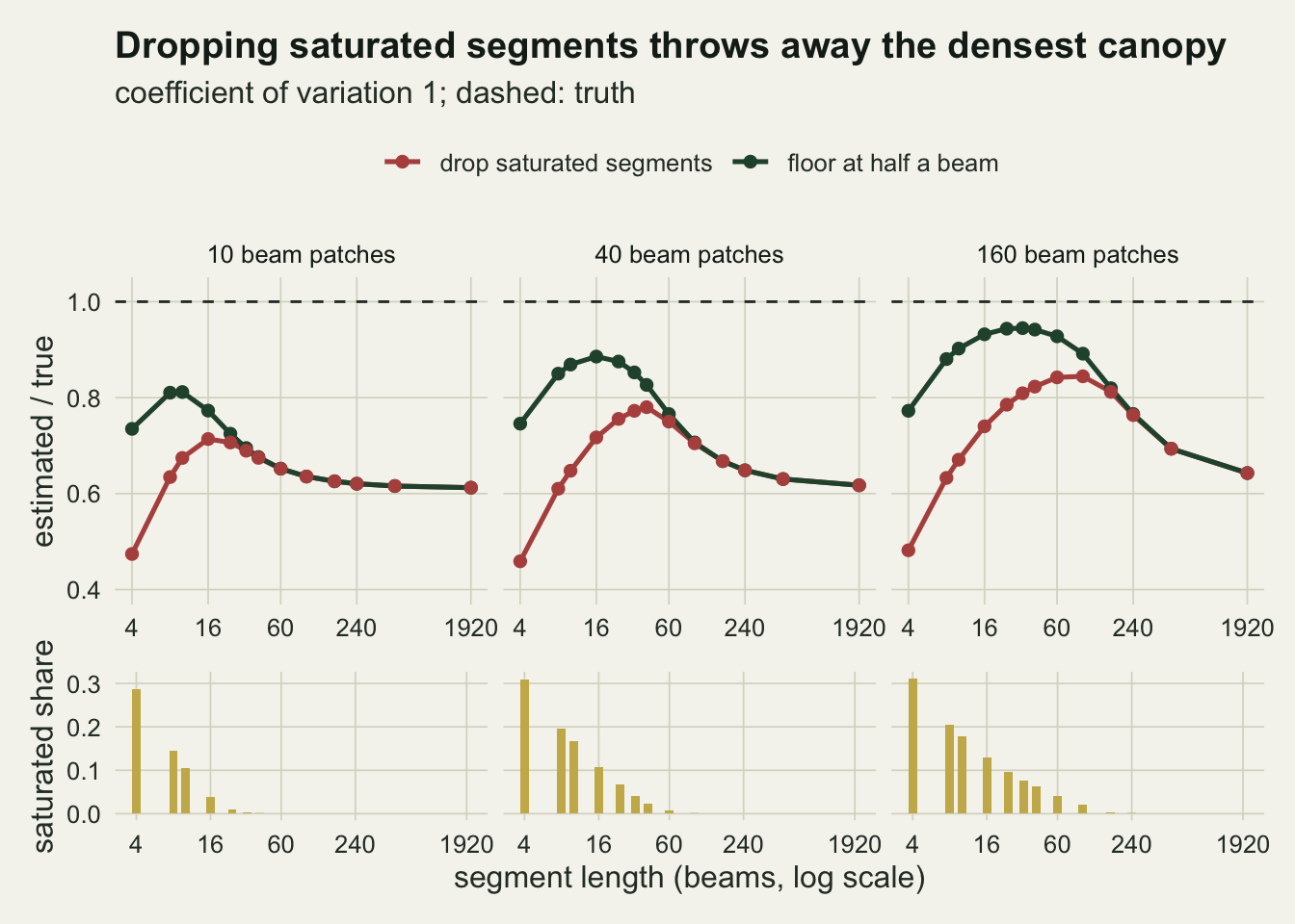
What to report
Report the estimator and the segment length together, and the rule for zero segments. An effective leaf area index from the log of a mean gap fraction, a Lang-Xiang average over segments of a stated length with a stated floor, and the same average with saturated segments dropped are three different quantities. On the strongly clumped canopy with 40-beam patches the log of the mean gave 0.617 of the truth, the best floored segment length 0.886, and dropping saturated 4-beam segments 0.459.
When the log of the mean is used, say so and give the closed form alongside it, or its equivalent for whatever canopy model is assumed. The ratio of 0.611 at a coefficient of variation of 1 is not a sampling error and does not shrink with more readings.
When segments are used, state the share of saturated segments. It is the one diagnostic available from the data themselves. In the sweep the two zero rules still disagreed by more than a hundredth at saturated shares between 0.7 and 2.1 per cent, so a share of that size or more means the reported value depends on a floor that was chosen, not measured.
Do not pick the segment length that gives the largest value, or the one that matches a destructive harvest on another site. The segment at which the estimator comes closest to the truth moved from 8 to 60 beams across patch sizes at moderate clumping, and did not exist at strong clumping, so a length tuned in one stand is not transferable. A gap-size correction of the kind Chen and Cihlar built into their clumping index uses the distribution of gap lengths along the transect rather than a segment length, and is the natural next step when the canopy is strongly clumped; Jonckheere and colleagues review it with the other indirect methods.
Honest limits
The canopy is one-dimensional and the simulated beam is vertical, so the 1/cos theta path-length term never enters. A real instrument integrates over zenith rings or a hemispherical image, where the path length through the canopy and the footprint of a segment both change with angle. The transect here stands in for a single vertical line of sight, not a zenith ring; it says how segment length interacts with clump size along one line of sight and nothing about how an analysis combines rings.
G was fixed at 0.5 and leaf angle was not simulated. Where leaf angle varies between crowns, G varies with it, and part of what appears here as clumping would appear instead as variation in projection. Woody area was ignored, so the truth is leaf area and the estimate contains only leaves; in a real stand stems and branches block beams and the optical estimate is of plant area.
Patch leaf area is gamma and constant inside a patch, with sharp edges. Crowns taper, and a tapered edge gives segments that straddle it a smoother mixture than the step used here, which probably moves the best segment length but was not measured. Patches were independent of each other; spatially correlated crowns would lengthen the effective clump scale.
The zero-segment rules are the two simple ones. The half-beam floor is a convention chosen for this post. It is not a description of any instrument or software package, and the post does not check how those handle saturated cells; the rule comparison shows why that choice has to be read from their documentation before a value is reported. The clumping-index correction was not implemented, so the post does not say how much of the strongly clumped gap it recovers.
Beams within a patch were independent Bernoulli trials. Leaves inside a crown are themselves clumped into shoots and branches, which adds within-segment clumping that no segment length can remove.
References
Nilson T 1971 Agricultural Meteorology 8:25-38 (10.1016/0002-1571(71)90092-6)
Lang ARG, Xiang Y 1986 Agricultural and Forest Meteorology 37(3):229-243 (10.1016/0168-1923(86)90033-X)
Chen JM, Cihlar J 1995 Applied Optics 34(27):6211-6222 (10.1364/AO.34.006211)
Jonckheere I, Fleck S, Nackaerts K, Muys B, Coppin P, Weiss M, Baret F 2004 Agricultural and Forest Meteorology 121(1-2):19-35 (10.1016/j.agrformet.2003.08.027)