library(ggplot2)

te_paper  <- "#f5f4ee"
te_ink    <- "#16241d"
te_body   <- "#2c3a31"
te_forest <- "#275139"
te_rust   <- "#b5534e"
te_line   <- "#dad9ca"

theme_datasheet <- function() {
  theme_minimal(base_size = 12) +
    theme(plot.background  = element_rect(fill = te_paper, colour = NA),
          panel.background = element_rect(fill = te_paper, colour = NA),
          panel.grid.major = element_line(colour = te_line, linewidth = 0.3),
          panel.grid.minor = element_blank(),
          text             = element_text(colour = te_body),
          plot.title       = element_text(colour = te_ink, face = "bold"),
          axis.text        = element_text(colour = te_body))
}

set.seed(20260813)Estimating plant cover with point intercepts
R
survey design
vegetation
statistics
ecology tutorial
A 100-pin frame is not 100 independent samples. Simulation shows how patchy vegetation shrinks the effective sample size and sinks the interval’s coverage.
Corrected 14 October 2026: the sentence that introduces the design effect called it the ratio of the patchy plot’s variance to the scattered plot’s; it now names the binomial variance as the denominator, which is what the code divides by.
Corrected 1 October 2026: the opening put the division by the number of pins outside the square root of the binomial standard error, and now puts it inside; the closing section described the frame as lying across a number of vegetation stretches, and now says how many times the length-weighted stretch the frame spans.
A hundred pins go down through the sward on a frame, forty of them touch Festuca, and the field sheet records 40 per cent cover. Then someone asks for an error bar, and the reflex is the binomial one: take p times one minus p, divide by the number of pins, and take the square root.
That formula assumes the hundred pins were a hundred independent looks at the plot. They were not. The pins sit 10 cm apart in a rigid frame, and grass grows in patches wider than the spacing between the pins, so a pin that lands in a tussock has neighbours that land in the same tussock. The frame asks the plot a hundred questions and gets back rather fewer than a hundred independent answers.
The estimate itself survives all of this. Point intercepts are unbiased under patchiness, however severe it gets. What breaks is everything downstream of the variance: the standard error, the interval, the weight the estimate carries in a model. This post builds a plot whose cover is known exactly, drops frames on it, and measures how often a nominal 95 per cent interval contains the truth.
Two plots with the same cover
To separate arrangement from amount we need two plots that differ only in arrangement. The first is a smoothed Gaussian field cut at a threshold, which gives patches of a controllable size. The second is the first one with its cells shuffled. No sward looks like that: it is not an alternative vegetation type but the arrangement the binomial formula quietly assumes, and it is here as the arithmetic reference. Same cells, same count, same cover down to the last cell: only the arrangement differs, so anything that separates the two afterwards was caused by pattern and nothing else.
nside    <- 512L        # cells per side; a 5 cm cell makes this a 25.6 m plot
p_target <- 0.35

# white noise smoothed with a Gaussian kernel, on a torus so there are no edges
smooth_noise <- function(nside, sigma) {
  dd <- pmin(0:(nside - 1), nside - 0:(nside - 1))
  gk <- exp(-dd^2 / (2 * sigma^2))
  Re(fft(fft(matrix(rnorm(nside * nside), nside, nside)) * fft(outer(gk, gk)),
         inverse = TRUE))
}

zz        <- smooth_noise(nside, sigma = 2)          # Gaussian kernel sd of 2 cells
clumped   <- (zz >= quantile(zz, 1 - p_target)) * 1L
scattered <- matrix(sample(clumped), nside, nside)   # the same cells, shuffled
p_true    <- mean(clumped)

c(patchy = mean(clumped), scattered = mean(scattered))
patchy scattered
0.3500023 0.3500023 The two plots hold the identical amount of vegetation. How coarse the patchy one came out is a separate question, and the kernel setting does not answer it. What decides everything below is how far the correlation between two cells reaches, and that can be measured on the field itself.
# correlation between the field and a copy of itself shifted k cells, both axes
shift_cor <- function(fld, k) {
  jj <- c((k + 1):nrow(fld), seq_len(k))
  0.5 * (cor(as.vector(fld), as.vector(fld[jj, ])) +
         cor(as.vector(fld), as.vector(fld[, jj])))
}

gaps  <- c(1L, 2L, 3L, 4L, 5L, 6L, 7L, 8L, 10L, 12L)
rho   <- sapply(gaps, function(k) shift_cor(clumped, k))
reach <- 5 * min(gaps[rho < 0.05])
runs  <- unlist(apply(clumped, 1, function(r) with(rle(r), lengths[values == 1L])))

print(round(setNames(rho, paste0(5 * gaps, "cm")), 3))
5cm 10cm 15cm 20cm 25cm 30cm 35cm 40cm 50cm 60cm
0.770 0.555 0.369 0.222 0.117 0.053 0.020 0.006 0.002 -0.001 round(c(reach_cm = reach,
mean_run_cm = 5 * mean(runs),
weighted_run_cm = 5 * sum(runs^2) / sum(runs)), 1) reach_cm mean_run_cm weighted_run_cm
35.0 33.0 49.2 Two cells 10 cm apart, the spacing the frame will use, agree far more often than chance: their correlation is 0.56, and it does not fall below 0.05 until 35 cm. An unbroken stretch of vegetation along a row runs 49 cm when the stretches are weighted by their length, which is what a pin dropped at random meets. The kernel’s standard deviation was two cells, one pin spacing, and the pattern it produced reaches 3.5 times that far: the setting and the grain are not the same number, and it is the grain that everything below depends on.
Onto each plot we drop a frame of 10 by 10 pins on a 10 cm spacing, so the frame is 90 cm across and covers a small fraction of the plot. Placement is uniform at random with wrap-around at the plot boundary, which makes every pin an equal-probability draw from the plot and removes any edge effect from the argument.
win  <- 60L                                  # a 3 m window at 5 cm cells
cell <- 0.05
idx  <- seq_len(win)

window_df <- function(fld, nm)
  data.frame(x = rep(idx, win) * cell, y = rep(idx, each = win) * cell,
             veg = factor(as.vector(fld[idx, idx]), levels = c(0, 1),
                          labels = c("bare", "plant")),
             field = nm)

maps   <- rbind(window_df(clumped, "patchy"), window_df(scattered, "scattered"))
pin_ij <- as.matrix(expand.grid(i = 21 + 2 * (0:9), j = 21 + 2 * (0:9)))
pins   <- data.frame(x = pin_ij[, 1] * cell, y = pin_ij[, 2] * cell)

ggplot(maps, aes(x = x, y = y)) +
  geom_raster(aes(fill = veg)) +
  geom_point(data = pins, colour = te_rust, size = 0.8) +
  scale_fill_manual(values = c(bare = te_line, plant = te_forest)) +
  coord_equal() +
  facet_wrap(~ field) +
  labs(x = "metres", y = "metres", fill = NULL,
       title = "Same cover, different arrangement, same pins") +
  theme_datasheet() +
  theme(legend.position = "bottom")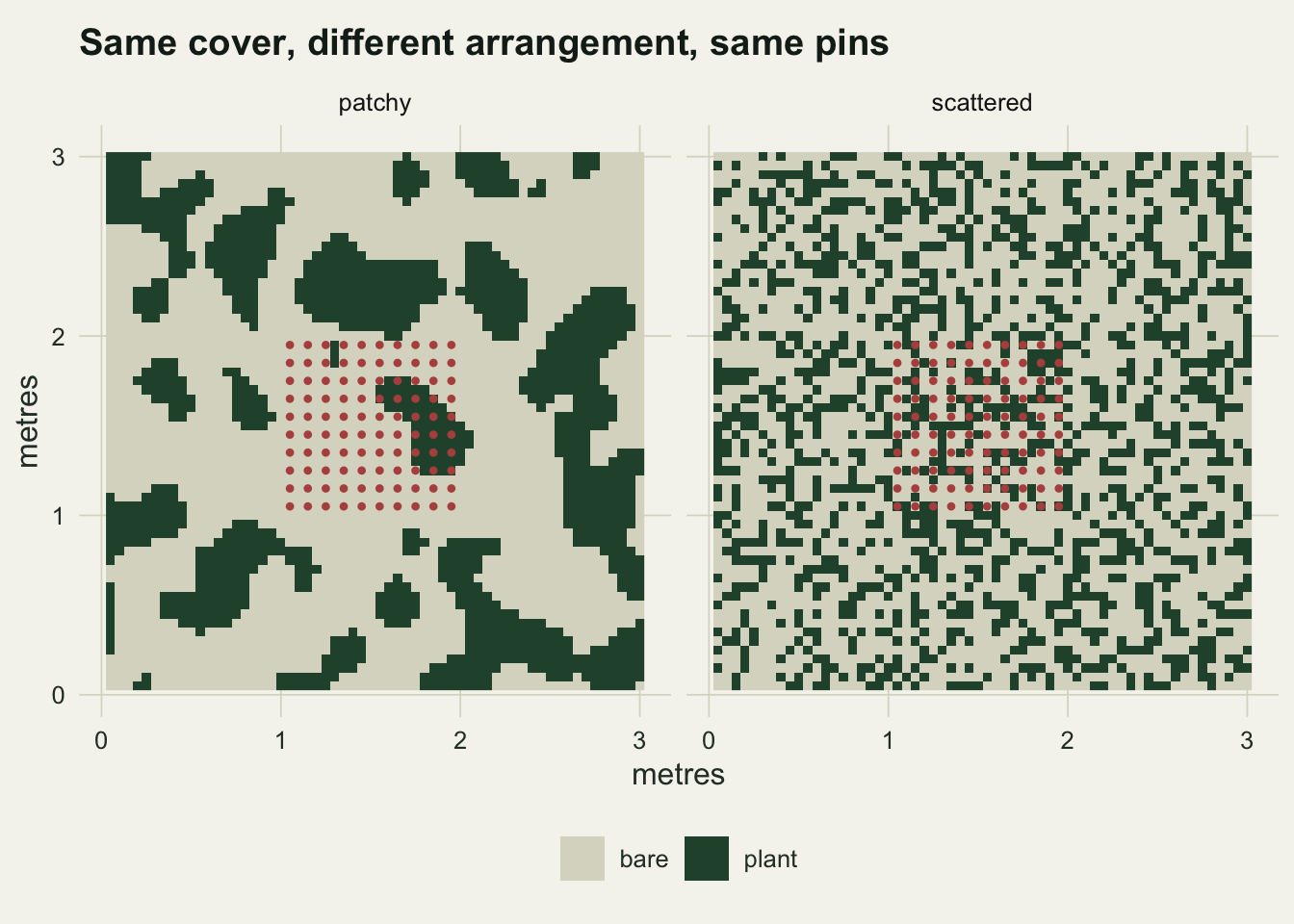
The left panel is why the binomial formula is in trouble. This frame has landed mostly on open ground, with one mass of vegetation covering the right-hand part of the grid, so long runs of pins along a row all say the same thing. It is an empty draw by this plot’s standards: 16 hits out of 100 against 35 per cent cover. Knowing the outcome of one pin tells you a good deal about its neighbour. In the right panel it tells you nothing.
The mean is right, the spread is not
Drop 20000 frames on each plot and look at what comes back.
pin_grid <- function(side, step)
  expand.grid(dx = step * (0:(side - 1)), dy = step * (0:(side - 1)))

drop_frames <- function(fld, pins, nframes) {
  nside <- nrow(fld)
  ox <- sample.int(nside, nframes, replace = TRUE) - 1L
  oy <- sample.int(nside, nframes, replace = TRUE) - 1L
  ix <- outer(ox, pins$dx, "+") %% nside + 1L
  iy <- outer(oy, pins$dy, "+") %% nside + 1L
  rowMeans(matrix(fld[cbind(as.vector(ix), as.vector(iy))], nrow = nframes))
}

frame100 <- pin_grid(10L, 2L)            # 10 x 10 pins, two cells (10 cm) apart
npin     <- nrow(frame100)
reps     <- 20000L
ph_clump <- drop_frames(clumped,   frame100, reps)
ph_scat  <- drop_frames(scattered, frame100, reps)

binom_var <- p_true * (1 - p_true) / npin
round(c(truth        = p_true,
        mean_patchy  = mean(ph_clump), mean_scattered = mean(ph_scat),
        sd_patchy    = sd(ph_clump),   sd_scattered   = sd(ph_scat),
        sd_binomial  = sqrt(binom_var)), 4)
truth mean_patchy mean_scattered sd_patchy sd_scattered
0.3500 0.3508 0.3499 0.1207 0.0481
sd_binomial
0.0477 Both means land on the truth. The patchy plot returns 0.3508 against a true cover of 0.3500, a gap smaller than the simulation’s own Monte Carlo standard error of 0.0009, and the scattered plot lands closer still. Patchiness does not bias point intercepts, and no amount of clumping will make it.
The two standard deviations are not the same number at all. The scattered plot delivers 0.0481, which is the binomial value to three decimal places, as it must be: on that plot the pins are independent draws by construction. The patchy plot delivers 0.1207, two and a half times larger. The ratio of a plot’s variance to the binomial one is the quantity survey statisticians call the design effect.
deff <- c(patchy = var(ph_clump), scattered = var(ph_scat)) / binom_var

wald_covers <- function(ph, n, truth) {
  se <- sqrt(ph * (1 - ph) / n)
  mean(ph - 1.96 * se <= truth & truth <= ph + 1.96 * se)
}

round(c(deff,
        n_eff_patchy    = npin / deff[["patchy"]],
        wald_patchy     = wald_covers(ph_clump, npin, p_true),
        wald_scattered  = wald_covers(ph_scat,  npin, p_true)), 3)
patchy scattered n_eff_patchy wald_patchy wald_scattered
6.404 1.015 15.616 0.529 0.940 The design effect on the patchy plot is 6.4. Divide the pin count by it and you get the effective sample size: those hundred pins carry about as much information about cover as 16 independent points would on the field drawn here, a figure that belongs to that draw rather than to the settings behind it. On the scattered plot the design effect is 1.02, which is one to within simulation noise, as it has to be when the pins really are independent.
The Wald interval does not know any of this. It computes its half-width from the pin count, so it produces the same width on both plots, and on the patchy plot it is far too small. Its measured coverage there is 0.529: an interval advertised at 95 per cent misses the truth about half the time. On the scattered plot the same interval covers 0.940 of the time, a shade under nominal for a reason that has nothing to do with pattern and everything to do with the Wald interval itself.
samp <- data.frame(phat  = c(ph_clump, ph_scat),
                   field = rep(c("patchy", "scattered"), each = reps))

ggplot(samp, aes(x = phat, fill = field)) +
  geom_histogram(aes(y = after_stat(density)), binwidth = 0.01,
                 boundary = 0.005, position = "identity", alpha = 0.6,
                 colour = NA) +
  geom_vline(xintercept = p_true, colour = te_ink, linewidth = 0.6) +
  geom_vline(xintercept = p_true + c(-1, 1) * 1.96 * sqrt(binom_var),
             linetype = "dashed", colour = te_body) +
  scale_fill_manual(values = c(patchy = te_rust, scattered = te_forest)) +
  labs(x = "cover estimated from one 100-pin frame", y = "density", fill = NULL,
       title = "The same estimator, two sampling distributions") +
  theme_datasheet() +
  theme(legend.position = "bottom")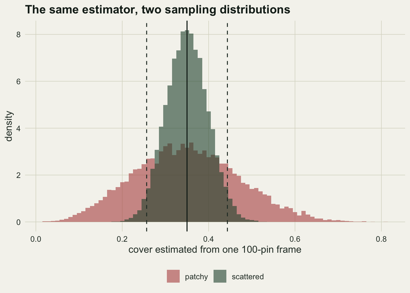
Spread the pins
The correlation lives inside the frame, so the first fix is to break the frame up. Keep the effort fixed at a hundred pins and vary how they are grouped: one frame of a hundred, four frames of twenty-five, twenty-five frames of four, or a hundred single pins dropped at independent locations.
survey_phat <- function(fld, side, nframes) {
  fr <- drop_frames(fld, pin_grid(side, 2L), nframes * reps)
  rowMeans(matrix(fr, nrow = reps, byrow = TRUE))
}

lay_ph <- list(ph_clump,                      # the single frame from above, reused
               survey_phat(clumped,  5L,   4L),
               survey_phat(clumped,  2L,  25L),
               survey_phat(clumped,  1L, 100L))

lay <- data.frame(pins_per_frame = c(100L, 25L, 4L, 1L),
                  frames         = c(1L, 4L, 25L, 100L),
                  se       = sapply(lay_ph, sd),
                  deff     = sapply(lay_ph, var) / binom_var,
                  coverage = sapply(lay_ph, wald_covers, n = npin, truth = p_true))
print(round(lay, 3))
pins_per_frame frames se deff coverage
1 100 1 0.121 6.404 0.529
2 25 4 0.111 5.370 0.573
3 4 25 0.075 2.475 0.767
4 1 100 0.047 0.979 0.944ggplot(lay, aes(x = pins_per_frame, y = coverage)) +
geom_hline(yintercept = 0.95, linetype = "dashed", colour = te_body) +
geom_line(colour = te_forest, linewidth = 0.9) +
geom_point(colour = te_rust, size = 3) +
scale_x_log10(breaks = lay$pins_per_frame) +
labs(x = "pins per frame (one hundred pins in total)",
y = "coverage of the nominal 95 per cent interval",
title = "The same pins, spread out") +
theme_datasheet()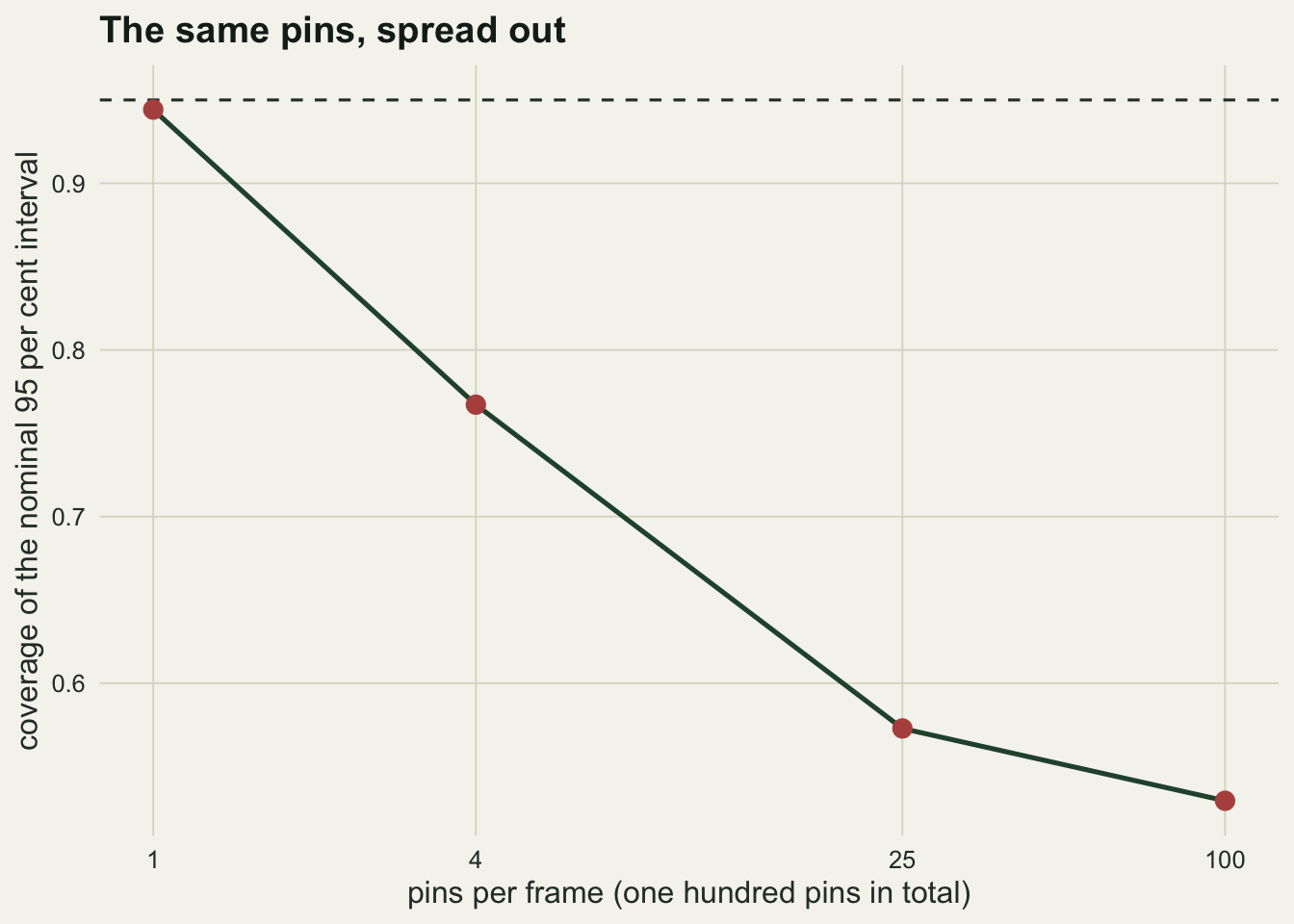
Going from one frame of a hundred to a hundred single pins drops the standard error from 0.121 to 0.047, a factor of 2.6, and takes the design effect from 6.4 to 0.98, which is one to within the same simulation noise, as a hundred pins dropped one at a time must be. Coverage recovers with it, from 0.53 to 0.94.
The middle of the table is where the lesson is. Four frames of twenty-five barely help: the design effect only falls to 5.4, because a 5 by 5 frame at 10 cm spacing is still 40 cm across, comparable with the patches themselves. Even frames of four pins, which span only 10 cm, carry a design effect of 2.5. The pins become independent only when they are dropped one at a time, far enough apart to miss each other’s patches. The design effect is a property of the frame relative to the grain of the vegetation, not of the frame alone.
The cost is walking. A hundred independent pin locations means a hundred stops instead of one, and in tall or wet vegetation the travel time dwarfs the reading time. That trade is the real design decision, and it is worth making with the design effect in front of you rather than by habit.
Take the variance from the frames
Sometimes the frame is fixed: it is the instrument the project owns, the protocol is already written, or the historic data came that way. The second fix does not touch the field method at all. It changes which units the variance is computed from.
Put ten frames of a hundred pins in the plot. The pin-level calculation treats this as a thousand independent Bernoulli draws. The alternative treats the ten frame-level cover values as the sample and takes their variance directly, which is what a survey statistician calls the ultimate-cluster estimator: the correlation inside a frame is already baked into that frame’s own estimate, so the spread between frames measures the true sampling variability without a model for it.
nfr      <- 10L
nsurv    <- 4000L
frame_ph <- matrix(drop_frames(clumped, frame100, nfr * nsurv),
                   nrow = nsurv, byrow = TRUE)
ph_big   <- rowMeans(frame_ph)                       # ten frames, 1000 pins
se_pin   <- sqrt(ph_big * (1 - ph_big) / (nfr * npin))
se_uc    <- apply(frame_ph, 1, sd) / sqrt(nfr)       # ultimate-cluster
tcrit    <- qt(0.975, nfr - 1)
cov_pin  <- mean(abs(ph_big - p_true) <= 1.96 * se_pin)
cov_uc   <- mean(abs(ph_big - p_true) <= tcrit * se_uc)

round(c(true_sd        = sd(ph_big),
        mean_se_pins   = mean(se_pin),
        mean_se_frames = mean(se_uc),
        cover_pins     = cov_pin,
        cover_frames   = cov_uc), 4)
true_sd mean_se_pins mean_se_frames cover_pins cover_frames
0.0376 0.0150 0.0372 0.5735 0.9495 Across 4000 simulated surveys the true standard deviation of this thousand-pin survey is 0.0376. The pin-level formula reports 0.0150 on average, understating it by a factor of about 2.5, and its interval covers 0.57. The frame-level formula reports 0.0372, which is the right size, and its interval covers 0.95, give or take a Monte Carlo margin of 0.007. Nothing was fitted and no correlation was estimated; the ten numbers were simply allowed to speak for themselves.
Two conditions come with it. There must be more than one frame, because one frame gives no variance estimate at all, and the frames must be placed independently rather than in a row along one edge of the plot. With ten frames the interval rests on nine degrees of freedom, so its width is itself an estimate; the t multiplier is what pays for that, and it is a fair price.
How far the design effect carries
A design effect of 6.4 is not a constant of nature. Two separate things move it: the grain of the vegetation, which the generator lets us dial, and the draw of the field, which moves the number with every setting held fixed.
new_field <- function(sigma) {
  z <- smooth_noise(nside, sigma)
  (z >= quantile(z, 1 - p_target)) * 1L
}

field_deff <- function(fld) {
  ph <- drop_frames(fld, frame100, reps)
  pp <- mean(fld)
  c(deff = var(ph) / (pp * (1 - pp) / npin), coverage = wald_covers(ph, npin, pp))
}

sweep_one <- function(sigma) {
  fl <- new_field(sigma)
  rr <- sapply(1:100, function(k) shift_cor(fl, k))
  c(kernel_cm   = 5 * sigma,
    rho_at_pins = shift_cor(fl, 2L),
    reach_cm    = 5 * which(rr < 0.05)[1],
    field_deff(fl))
}

swp <- as.data.frame(t(sapply(c(0.5, 1, 2, 4, 20), sweep_one)))
print(round(swp, 3))
kernel_cm rho_at_pins reach_cm deff coverage
1 2.5 0.010 10 1.030 0.937
2 5.0 0.234 20 2.196 0.789
3 10.0 0.566 35 7.618 0.495
4 20.0 0.772 65 21.515 0.277
5 100.0 0.951 250 76.009 0.059The middle columns are the ones to match against a real sward, because they can be measured there: the correlation between two pins a spacing apart, and the distance at which it dies. When it is gone by the pin spacing the design effect is 1.03 and coverage is near nominal at 0.94. Where it is still 0.95 at the pin spacing the design effect is 76, the hundred pins are worth 1.3 independent points, and coverage collapses to 0.06. Each row is one fresh field, which is why the third, drawn at this post’s own settings, reports 7.6 rather than 6.4.
dfs <- replicate(12L, field_deff(new_field(2))[["deff"]])

round(c(published = deff[["patchy"]], mean = mean(dfs), sd = sd(dfs),
        lowest = min(dfs), highest = max(dfs),
        below_published = sum(dfs < deff[["patchy"]])), 2)
published mean sd lowest highest
6.40 6.90 0.30 6.52 7.45
below_published
0.00 So the design effect is a property of the field as much as of the recipe. Twelve fresh fields at the same kernel, the same pins and the same target cover average 6.9 and run from 6.5 to 7.4, and the number landing as low as the field drawn here is 0: the 6.4 quoted above is the friendly end of its own distribution, and the sweep row above, a thirteenth draw at the same settings, sat a little beyond the other end. That spread, 0.30, is several times the Monte Carlo error of a single design effect, which at 20000 frames is of order 0.06. Redrawing the vegetation moves the answer further than running more frames does.
What a hundred pins can resolve
There is a floor underneath all of this that has nothing to do with correlation. With 100 pins the estimate can only take 101 distinct values, spaced 1 per cent apart. Across 20000 frames on the patchy plot the estimator produced 77 different numbers in total, every one a whole number of pins over a hundred. A change in cover smaller than one pin cannot be seen by one frame, and fitting beta regression to the difference between 0.37 and 0.38 is reading a single pin, the smallest step the instrument has.
One more caution about the interval itself. Many real cover values sit close to zero or close to one, which is where the Wald interval behaves worst: it runs past the boundary, and when no pin hits at all it collapses to zero width and claims perfect certainty. The Wilson interval is the better default there and costs nothing extra. Fixing the clustering does not fix the boundary, and the two problems usually arrive together.
Honest limits
A real pin frame does not record one hit per pin. It records every contact down the pin, by species and often by layer, so total cover summed across species routinely exceeds 100 per cent and a single species can be recorded at several heights. The simulation here gives each pin one Bernoulli outcome for one species, which is the simplest case and the one where the binomial reflex is most defensible. Multiple hits per pin add another layer of within-pin correlation on top of the between-pin correlation shown here, and they push in the same direction.
The design effect of 6.4 belongs to this grain of vegetation, this pin spacing, this cover value and this one draw of the field, and it does not transfer to your data. What transfers is the shape of the sweep above: pins whose correlation has run out by the spacing between them behave binomially, and every centimetre it reaches past that spacing is paid for in coverage. Here it is still 0.56 at the pin spacing and reaches 35 cm, so a 90 cm frame spans only about 1.8 times the length-weighted stretch of vegetation measured earlier. The number to report is the one you measure from your own frames, and the frame-level variance above is how you measure it.
An observer deciding whether the pin touched a leaf is a second error source, and the simulation gets that decision right for free. In the field, glancing contacts, leaf movement, pin diameter and the angle of the drop all enter, and they are correlated within an observer and within a frame in ways this simulation says nothing about. Disagreement of that sort does not average out over a survey where each observer does their own plots.
Frames here are placed uniformly at random on a torus, so the estimator has no edge effects and no systematic component. Real surveys often place frames systematically along a transect, which usually beats random placement for precision, and the frame-level variance estimator then tends to overstate the uncertainty rather than understate it. That is the safe direction to err in, but it is not the same thing as being correct.
Finally, the truth being estimated here is the cover of one simulated plot, held fixed while frames move over it. A study that wants a mean over many plots has a second level of variation on top, and the same argument applies again one level up: plots, not frames, become the sampling unit.
References
Goodall DW 1952 Australian Journal of Biological Sciences 5(1):1-41 (10.1071/BI9520001)
Bonham CD 2013 Measurements for Terrestrial Vegetation, second edition. Wiley-Blackwell. ISBN 978-0-470-97258-8
Agresti A, Coull BA 1998 The American Statistician 52(2):119-126 (10.1080/00031305.1998.10480550)
Brown LD, Cai TT, DasGupta A 2001 Statistical Science 16(2):101-133 (10.1214/ss/1009213286)
Damgaard C 2012 Ecology 93(6):1269-1274 (10.1890/11-1499.1)