library(ggplot2)
library(patchwork)

te_paper  <- "#f5f4ee"
te_ink    <- "#16241d"
te_body   <- "#2c3a31"
te_forest <- "#275139"
te_rust   <- "#b5534e"
te_gold   <- "#c9b458"
te_line   <- "#dad9ca"

theme_datasheet <- function() {
  theme_minimal(base_size = 12) +
    theme(plot.background  = element_rect(fill = te_paper, colour = NA),
          panel.background = element_rect(fill = te_paper, colour = NA),
          panel.grid.major = element_line(colour = te_line, linewidth = 0.3),
          panel.grid.minor = element_blank(),
          text             = element_text(colour = te_body),
          plot.title       = element_text(colour = te_ink, face = "bold"),
          plot.subtitle    = element_text(colour = te_body),
          axis.text        = element_text(colour = te_body))
}Curve registration and functional PCA
R
functional data
phenology
PCA
smoothing
ecology tutorial
Averaging shifted flowering curves flattens the peak. Registration in R by shift or pinned warp decides what a functional PCA of the season calls amplitude.
A meadow has been walked every four days through thirty flowering seasons, and on each visit the observer records the proportion of marked plants with open flowers. Each season gives a hump: a quick rise in late spring, a peak, a slower fade. The obvious summary of thirty humps is their average, drawn day by day, and the obvious next step is a principal component analysis of the thirty curves to see how seasons differ. Both steps are routine, and both go wrong in the same way when the seasons differ in timing.
The problem is that a curve varies in two different directions. It can be taller or shorter, which is amplitude variation, and it can come earlier or later, which is phase variation. A day by day average cannot tell the two apart. If one season peaks on day 170 and another on day 190, the average on day 180 mixes the rising limb of one with the falling limb of the other, and the resulting curve is wider and lower than either. The flattening is not noise; it is what phase variation turns into once it has been averaged over.
The site has met the phase and amplitude pair before, in a parametric form. Harmonic regression on a seasonal raster fits sine and cosine terms to every pixel, so amplitude and phase follow from the coefficients of one linear model, and the peak day is read off the fitted curve. That works when the season has the shape the harmonics can express. Here no shape is assumed: each season is smoothed without a phase parameter, so phase has to be removed from the curves themselves before they are compared, which is what registration does. Quantifying phenological mismatch is the other close neighbour, because it also treats a season as a curve rather than a date, but it compares two known Gaussian pulses and never has to estimate where a peak is.
The post does four things. It builds thirty seasons with known peaks, amplitudes and widths, and measures how much the pointwise mean loses. It registers the curves on their peaks in two ways, with a pure shift and with a piecewise linear warp whose ends are pinned to the observation window. It runs a functional principal component analysis before and after registration and checks what the first component describes under each warp. Last, it repeats the whole pipeline on many simulated sets of seasons and at several noise levels, because one set of thirty curves is one draw.
Thirty seasons with a known answer
Every season is a two-sided Gaussian hump: a peak height, a peak day, and a width that is shorter on the rising limb than on the falling one, because flowering usually opens faster than it fades. Across seasons the peak day varies with a standard deviation of twelve days, the peak height varies by about twenty per cent on the log scale, and the width varies a little too. Visits run every four days from day 100 to day 260, and each visit adds observation noise. All of these constants were fixed before anything was run and were not changed afterwards.
n_curve    <- 30
day_lo     <- 100
day_hi     <- 260
visit_step <- 4
obs_day    <- seq(day_lo, day_hi, by = visit_step)
grid_day   <- seq(day_lo, day_hi, by = 0.5)

peak_mid   <- 180     # mean peak day
peak_sd    <- 12      # between-season sd of the peak day
amp_mid    <- 0.6     # median peak proportion in flower
amp_logsd  <- 0.2     # between-season sd of log peak height
wid_mid    <- 14      # median width in days
wid_logsd  <- 0.15    # between-season sd of log width
rise_frac  <- 0.8     # rising limb width as a fraction of the width
fall_frac  <- 1.25    # falling limb width as a fraction of the width
noise_sd   <- 0.03    # observation noise, proportion in flower

season_hump <- function(d, amp, peak, wid) {
  side_w <- ifelse(d < peak, rise_frac, fall_frac) * wid
  amp * exp(-(d - peak)^2 / (2 * side_w^2))
}

sim_seasons <- function(noise = noise_sd) {
  amp  <- amp_mid * exp(rnorm(n_curve, 0, amp_logsd))
  peak <- peak_mid + rnorm(n_curve, 0, peak_sd)
  wid  <- wid_mid * exp(rnorm(n_curve, 0, wid_logsd))
  obs  <- t(vapply(seq_len(n_curve), function(i)
    season_hump(obs_day, amp[i], peak[i], wid[i]) +
      rnorm(length(obs_day), 0, noise), numeric(length(obs_day))))
  truth <- t(vapply(seq_len(n_curve), function(i)
    season_hump(grid_day, amp[i], peak[i], wid[i]), numeric(length(grid_day))))
  list(amp = amp, peak = peak, wid = wid, obs = obs, truth = truth)
}

smooth_seasons <- function(obs) {
  t(apply(obs, 1, function(y) predict(smooth.spline(obs_day, y), grid_day)$y))
}

set.seed(4127)
seasons  <- sim_seasons()
fit_curv <- smooth_seasons(seasons$obs)
n_visit  <- length(obs_day)
Each season has 41 visits. Each is smoothed on its own with smooth.spline(), which picks its smoothing parameter by generalised cross-validation, and the smooth is evaluated on a half-day grid. From here on the curves are the data: thirty rows of a matrix, one column per half day.
The pointwise mean is a flattened season
ind_peak  <- apply(fit_curv, 1, max)
mean_un   <- colMeans(fit_curv)
peak_un   <- max(mean_un)
loss_un   <- 100 * (1 - peak_un / mean(ind_peak))
frac_high <- mean(ind_peak > peak_un)
n_high    <- sum(ind_peak > peak_un)
wide_un   <- sum(mean_un > peak_un / 2) * 0.5
wide_each <- apply(fit_curv, 1, function(y) sum(y > max(y) / 2)) * 0.5
wide_ind  <- mean(wide_each)
n_wider   <- sum(wide_each >= wide_un)
n_low     <- n_curve - sum(ind_peak > peak_un)

wid_side  <- wid_mid * (rise_frac + fall_frac) / 2
gauss_red <- 100 * (1 - wid_side / sqrt(wid_side^2 + peak_sd^2))
The thirty smoothed seasons peak at 0.570 of plants in flower on average. The day by day mean of the same thirty curves peaks at 0.452, which is 20.8 per cent lower. The mean curve is also wider: it stays above half of its own peak for 44.5 days, while the individual seasons do so for 35.3 days on average.
The loss has a simple source. If every season had the same symmetric Gaussian shape with width w, and peak days were normal with standard deviation s, the pointwise mean would be another Gaussian with width the square root of w squared plus s squared, and its height would drop by the factor w over that square root. Using the average of the two limb widths, 14.35 days, and the design value of s, that approximation predicts a loss of 23.3 per cent. The flattening is set by the ratio of timing spread to curve width, not by the number of seasons, so it does not shrink as more seasons are added.
The mean curve is not lower than every season, though. Peak heights vary too, and 27 of the 30 seasons (90 per cent) peak above the mean curve. The 3 seasons under it are simply the ones with the lowest peaks. Its width is the more telling number: only 3 of the 30 seasons are as wide at half height as the mean curve. What the mean describes is a low, broad season that few of the real seasons resemble.
Registering on the peak
Landmark registration picks a feature that every curve has, here the peak, and moves each curve along the time axis so that the feature lands at the same place for all of them. Kneip and Gasser set out the landmark approach in 1992. The landmark fixes one point of the warp; the rest of the warp is a choice, and two common choices are compared here.
The first is a pure shift: every season is slid along the time axis by the distance between its estimated peak and the mean estimated peak, so the whole curve moves and keeps its shape. The second is a piecewise linear warp with pinned ends: the start and end of the observation window, days 100 and 260, stay where they are, the estimated peak is mapped to the mean peak day, and time is stretched linearly on each side. The pinned warp is the natural one when every season has to fill the same window, and it is what a landmark registration with the window ends as extra landmarks gives.
Only one of them matches the simulation. In season_hump() the peak day enters only through the difference between the day and the peak, so a later season is the same hump moved later. Timing in these data is a translation, and the shift is the correct warp family for them. The pinned warp is misspecified: a season that peaked late has its rising limb compressed and its falling limb stretched, and an early season the reverse. A registered curve is in both cases the smoothed curve read off at warped time.
register_peak <- function(fit) {
  pk_hat <- grid_day[apply(fit, 1, which.max)]
  pk_ref <- mean(pk_hat)
  warp   <- t(vapply(seq_len(nrow(fit)), function(i)
    ifelse(grid_day <= pk_ref,
           day_lo + (grid_day - day_lo) * (pk_hat[i] - day_lo) / (pk_ref - day_lo),
           pk_hat[i] + (grid_day - pk_ref) * (day_hi - pk_hat[i]) / (day_hi - pk_ref)),
    numeric(length(grid_day))))
  reg <- t(vapply(seq_len(nrow(fit)), function(i)
    approx(grid_day, fit[i, ], xout = warp[i, ])$y, numeric(length(grid_day))))
  list(reg = reg, warp = warp, pk_hat = pk_hat, pk_ref = pk_ref)
}

# pure shift; beyond the window the curve is held at its end value
shift_peak <- function(fit, pk_hat = grid_day[apply(fit, 1, which.max)]) {
  pk_ref <- mean(pk_hat)
  t(vapply(seq_len(nrow(fit)), function(i)
    approx(grid_day, fit[i, ], xout = grid_day + pk_hat[i] - pk_ref,
           rule = 2)$y, numeric(length(grid_day))))
}

reg_out  <- register_peak(fit_curv)
wp_curv  <- reg_out$reg
sh_curv  <- shift_peak(fit_curv)
mean_wp  <- colMeans(wp_curv)
mean_sh  <- colMeans(sh_curv)
peak_wp  <- max(mean_wp)
peak_sh  <- max(mean_sh)
loss_wp  <- 100 * (1 - peak_wp / mean(ind_peak))
loss_sh  <- 100 * (1 - peak_sh / mean(ind_peak))
edge_max <- max(abs(fit_curv[, c(1, length(grid_day))]))
bias_wp  <- 100 * (peak_wp / mean(seasons$amp) - 1)
bias_sh  <- 100 * (peak_sh / mean(seasons$amp) - 1)
bias_sm  <- 100 * (mean(ind_peak) / mean(seasons$amp) - 1)
wide_wp  <- sum(mean_wp > peak_wp / 2) * 0.5
wide_sh  <- sum(mean_sh > peak_sh / 2) * 0.5
on_grid  <- reg_out$pk_ref %in% grid_day

pk_err_sd  <- sd(reg_out$pk_hat - seasons$peak)
pk_err_max <- max(abs(reg_out$pk_hat - seasons$peak))
var_un     <- sum(apply(fit_curv, 2, var))
var_left_wp <- 100 * sum(apply(wp_curv, 2, var)) / var_un
var_left_sh <- 100 * sum(apply(sh_curv, 2, var)) / var_un

# how the pinned warp rescales the limbs of a season one sd late
late_pk   <- reg_out$pk_ref + peak_sd
late_rise <- (reg_out$pk_ref - day_lo) / (late_pk - day_lo)
late_fall <- (day_hi - reg_out$pk_ref) / (day_hi - late_pk)

half_width <- function(mat, side) apply(mat, 1, function(y) {
  top <- which.max(y)
  keep <- if (side == "rise") seq_len(top) else top:length(y)
  sum(y[keep] > max(y) / 2) * 0.5
})
r_rise_un <- cor(half_width(fit_curv, "rise"), seasons$peak)
r_rise_sh <- cor(half_width(sh_curv, "rise"), seasons$peak)
r_rise_wp <- cor(half_width(wp_curv, "rise"), seasons$peak)
r_fall_sh <- cor(half_width(sh_curv, "fall"), seasons$peak)
r_fall_wp <- cor(half_width(wp_curv, "fall"), seasons$peak)
The estimated peak days miss the true ones with a standard deviation of 1.09 days and never by more than 3.5 days, so the landmark itself is well determined at this visit spacing and noise. Both registrations use the same estimated peaks.
After registration the mean curve peaks at 0.570 with the shift and at 0.570 with the pinned warp, losses of 0.016 and 0.016 per cent against the mean of the individual peaks. That near zero (not exactly zero, because the reference day falls between grid points) is guaranteed by construction and is no evidence of anything: near the reference day every registered curve sits at its own maximum, so the mean there is the mean of the maxima. The comparison that means something is against the truth. The registered mean peak is 1.3 per cent below the mean true peak height with the shift and 1.3 per cent with the warp, and that shortfall is already present before registration: the smoothed individual peaks are 1.3 per cent below their true heights, because a smoothing spline shaves the top off a hump. The registered mean is 34.5 days wide at half height after the shift and 34.5 days after the warp, the same to the half-day grid, against 35.3 days for the average season.
At the peak the two registrations agree, and the difference is in the limbs. For a season peaking one standard deviation late, the pinned warp multiplies the rising limb by 0.87 and the falling limb by 1.18. That is a width change of the same order as the design’s between-season width variation (a standard deviation of 0.15 on the log scale), and unlike that variation it is tied to timing. On this set the rising half-width of the registered curves correlates with the true peak day at -0.74 after the pinned warp, against -0.19 after the shift and -0.16 before registration; the falling half-width correlates at 0.46 after the warp and -0.23 after the shift. The warp takes timing out of the peak position and puts some of it back into the shape.
The same thing shows in how much variance registration removes. Summed over the grid, the variance between registered curves is 22.0 per cent of the variance between the unregistered ones after the shift and 27.1 per cent after the pinned warp. The rest was removed by the warp, and the two warps remove different amounts from the same curves.
curve_long <- function(mat, lab) {
  data.frame(day = rep(grid_day, each = nrow(mat)),
             value = as.vector(mat),
             season = rep(seq_len(nrow(mat)), times = length(grid_day)),
             panel = lab)
}
panel_lab <- c("as recorded", "registered: shift", "registered: pinned warp")
mean_long <- rbind(data.frame(day = grid_day, value = mean_un, panel = panel_lab[1]),
                   data.frame(day = grid_day, value = mean_sh, panel = panel_lab[2]),
                   data.frame(day = grid_day, value = mean_wp, panel = panel_lab[3]))
curves_df <- rbind(curve_long(fit_curv, panel_lab[1]),
                   curve_long(sh_curv, panel_lab[2]),
                   curve_long(wp_curv, panel_lab[3]))
curves_df$panel <- factor(curves_df$panel, levels = panel_lab)
mean_long$panel <- factor(mean_long$panel, levels = panel_lab)
ref_df <- data.frame(panel = factor(panel_lab, levels = panel_lab),
                     y = mean(ind_peak))

ggplot(curves_df, aes(day, value)) +
  geom_line(aes(group = season), colour = te_forest, alpha = 0.35,
            linewidth = 0.45) +
  geom_hline(data = ref_df, aes(yintercept = y), linetype = "dashed",
             colour = te_ink, linewidth = 0.5) +
  geom_line(data = mean_long, colour = te_rust, linewidth = 1.3) +
  facet_wrap(~ panel, ncol = 1) +
  coord_cartesian(xlim = c(130, 240)) +
  labs(x = "day of year", y = "proportion of plants in flower",
       title = "Averaging over timing lowers and widens the peak",
       subtitle = "green: thirty seasons; red: day by day mean; dashed: mean of the individual peaks") +
  theme_datasheet() +
  theme(strip.text = element_text(colour = te_ink, face = "bold", hjust = 0))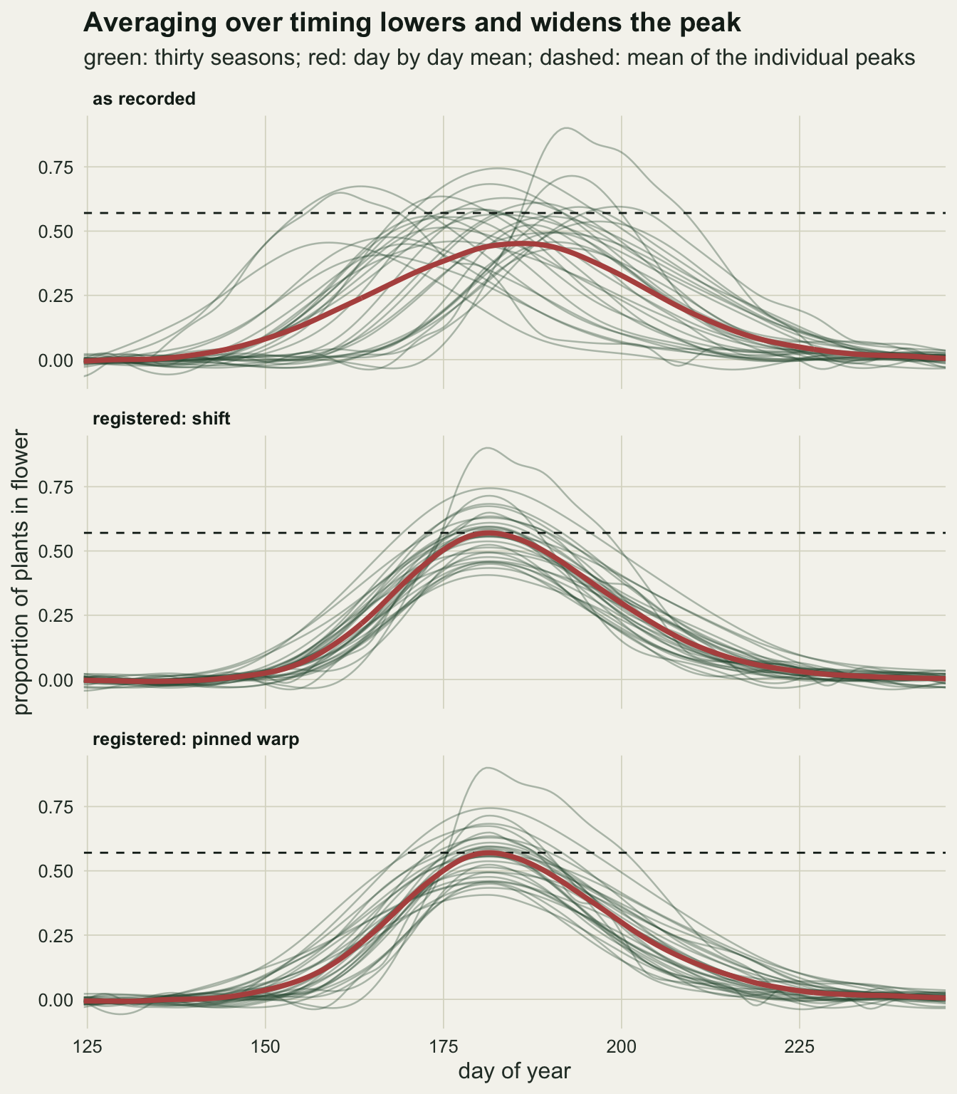
Functional PCA before and after
Functional principal component analysis is ordinary principal component analysis applied to curves evaluated on a fine grid, with each column a time point. Ramsay and Silverman compute it from a basis expansion, optionally with a roughness penalty on the components. Without the penalty, on a dense evenly spaced grid, prcomp() on the centred curve matrix gives the same components: the quadrature weight is a constant h of 0.5 day, so the functions are the loadings divided by the square root of h, the variances are multiplied by h, and the shares do not change. The question is what the first component describes.
A shift in time has a known signature. If a curve is moved later by a small amount, the change at each day is approximately minus the slope of the curve at that day. So a component that encodes timing should look like the slope of the mean curve up to sign; drawn as minus the slope, as below, it is negative on the rising limb and positive on the falling limb. A component that encodes height should look like the mean curve itself.
pc_un <- prcomp(fit_curv)
pc_sh <- prcomp(sh_curv)
pc_wp <- prcomp(wp_curv)
share_of <- function(pc, k = 1) pc$sdev[k]^2 / sum(pc$sdev^2)

slope_un <- c(diff(mean_un), NA) / 0.5
slope_sh <- c(diff(mean_sh), NA) / 0.5
slope_wp <- c(diff(mean_wp), NA) / 0.5
ok_idx   <- seq_len(length(grid_day) - 1)

orient <- function(load, ref) if (cor(load, ref, use = "complete.obs") < 0) -1 else 1
sign_un  <- orient(pc_un$rotation[, 1], -slope_un)
sign_sh  <- orient(pc_sh$rotation[, 1], mean_sh)
sign_wp  <- orient(pc_wp$rotation[, 1], mean_wp)
load_un  <- sign_un * pc_un$rotation[, 1]
load_sh  <- sign_sh * pc_sh$rotation[, 1]
load_wp  <- sign_wp * pc_wp$rotation[, 1]
score_un <- sign_un * pc_un$x[, 1]
score_sh <- sign_sh * pc_sh$x[, 1]
score_wp <- sign_wp * pc_wp$x[, 1]

sh_un  <- 100 * share_of(pc_un)
sh_sh  <- 100 * share_of(pc_sh)
sh_wp  <- 100 * share_of(pc_wp)
sh2_un <- 100 * share_of(pc_un, 2)

r_un_slope <- cor(load_un[ok_idx], -slope_un[ok_idx])
r_un_mean  <- cor(load_un, mean_un)
r_sh_mean  <- cor(load_sh, mean_sh)
r_sh_slope <- cor(load_sh[ok_idx], -slope_sh[ok_idx])
r_wp_mean  <- cor(load_wp, mean_wp)
r_wp_slope <- cor(load_wp[ok_idx], -slope_wp[ok_idx])

r_score_pk <- cor(score_un, seasons$peak)
r_un_amp   <- cor(score_un, seasons$amp)
r_un2_amp  <- abs(cor(pc_un$x[, 2], seasons$amp))
r_sh_amp   <- cor(score_sh, seasons$amp)
r_wp_amp   <- cor(score_wp, seasons$amp)
r_sh_wid   <- cor(score_sh, seasons$wid)
r_wp_wid   <- cor(score_wp, seasons$wid)
r_sh_pk    <- cor(score_sh, seasons$peak)
r_wp_pk    <- cor(score_wp, seasons$peak)
r_wp_pkhat <- cor(score_wp, reg_out$pk_hat)
fall_day   <- 205
fall_ld_sh <- load_sh[grid_day == fall_day] / max(load_sh)
fall_ld_wp <- load_wp[grid_day == fall_day] / max(load_wp)
fall_mean  <- mean_sh[grid_day == fall_day] / max(mean_sh)
Before registration the first component explains 69.3 per cent of the variance and the second 18.9 per cent. After the shift the first component explains 66.1 per cent, and after the pinned warp 56.3 per cent. On this set both registrations lower the share, the warp by far more than the shift. Whether that is typical is a question for the replicates below; what one set already shows is that the share depends on the warp as much as on the curves.
The loadings tell a clearer story than the shares. The unregistered first component correlates at 0.951 with minus the slope of the mean curve and at 0.191 with the mean curve itself: it is the derivative-shaped timing mode. After the shift the first component correlates at 0.932 with its mean curve and at 0.113 with minus the slope; after the pinned warp the figures are 0.904 and 0.308. Both are mainly height modes. Neither matches the mean curve on the falling limb: the loading stays high after the peak, at 0.80 of its maximum on day 205 after the shift and 0.87 after the warp, where the mean curve is down to 0.37 of its peak. Most of that shoulder is the simulated width variation, which acts most on the longer falling limb; the warp adds a little to it.
rescale_to <- function(v, target) v / max(abs(v), na.rm = TRUE) * max(abs(target))
load_panel <- c("as recorded: against minus the slope of the mean",
                "shift: against the mean curve",
                "pinned warp: against the mean curve")
load_df <- rbind(
  data.frame(day = grid_day, value = load_un, what = "first component",
             panel = load_panel[1]),
  data.frame(day = grid_day, value = rescale_to(-slope_un, load_un),
             what = "reference shape", panel = load_panel[1]),
  data.frame(day = grid_day, value = load_sh, what = "first component",
             panel = load_panel[2]),
  data.frame(day = grid_day, value = rescale_to(mean_sh, load_sh),
             what = "reference shape", panel = load_panel[2]),
  data.frame(day = grid_day, value = load_wp, what = "first component",
             panel = load_panel[3]),
  data.frame(day = grid_day, value = rescale_to(mean_wp, load_wp),
             what = "reference shape", panel = load_panel[3]))
load_df$panel <- factor(load_df$panel, levels = load_panel)

ggplot(load_df[!is.na(load_df$value), ], aes(day, value, colour = what,
                                             linetype = what)) +
  geom_hline(yintercept = 0, colour = te_line, linewidth = 0.5) +
  geom_line(linewidth = 1) +
  facet_wrap(~ panel, ncol = 1, scales = "free_y") +
  scale_colour_manual(values = c(te_forest, te_rust), name = NULL) +
  scale_linetype_manual(values = c("solid", "dashed"), name = NULL) +
  coord_cartesian(xlim = c(130, 240)) +
  labs(x = "day of year", y = "loading",
       title = "The same first component, different jobs",
       subtitle = "before registration a timing mode; after either registration, mainly a height mode") +
  theme_datasheet() +
  theme(legend.position = "bottom",
        strip.text = element_text(colour = te_ink, face = "bold", hjust = 0))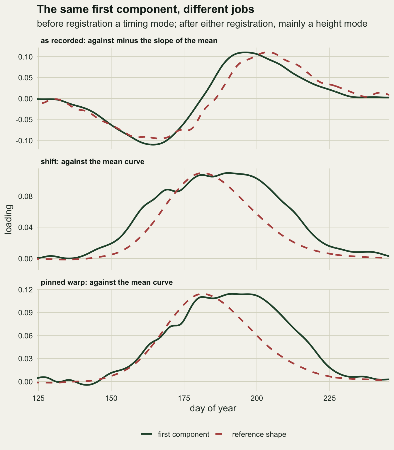
Because the seasons were simulated, the component scores can be checked against what generated them. The unregistered first score correlates at 0.976 with the true peak day and at 0.336 with the true peak height. Before registration the height signal is split: the first score still carries some of it, and the second score correlates at 0.513 in absolute value with peak height, mixed with whatever second-order timing effects the linear shift approximation leaves over.
After the shift the first score correlates at 0.806 with the true peak height, 0.521 with the true width and 0.080 with the true peak day. After the pinned warp the same three correlations are 0.851, 0.420 and 0.268. The last number is the leak: the peak day has been registered away, yet the first “amplitude” score of the warped curves still tracks it, through the limb stretching described above. Against the estimated peak days, which a real analysis has, the correlation is 0.246. Thirty seasons give a noisy correlation, so the replicates below say whether the difference is real.
p_left <- ggplot(data.frame(x = seasons$peak, y = score_un), aes(x, y)) +
  geom_point(colour = te_forest, size = 2.2) +
  labs(x = "true peak day", y = "first component score",
       title = "As recorded",
       subtitle = sprintf("r = %.2f with peak day", r_score_pk)) +
  theme_datasheet()
p_right <- ggplot(data.frame(x = seasons$amp, y = score_sh), aes(x, y)) +
  geom_point(colour = te_rust, size = 2.2) +
  labs(x = "true peak proportion in flower", y = "first component score",
       title = "Registered by a shift",
       subtitle = sprintf("r = %.2f with peak height", r_sh_amp)) +
  theme_datasheet()
p_left + p_right +
  plot_annotation(theme = theme(plot.background = element_rect(fill = te_paper, colour = NA)))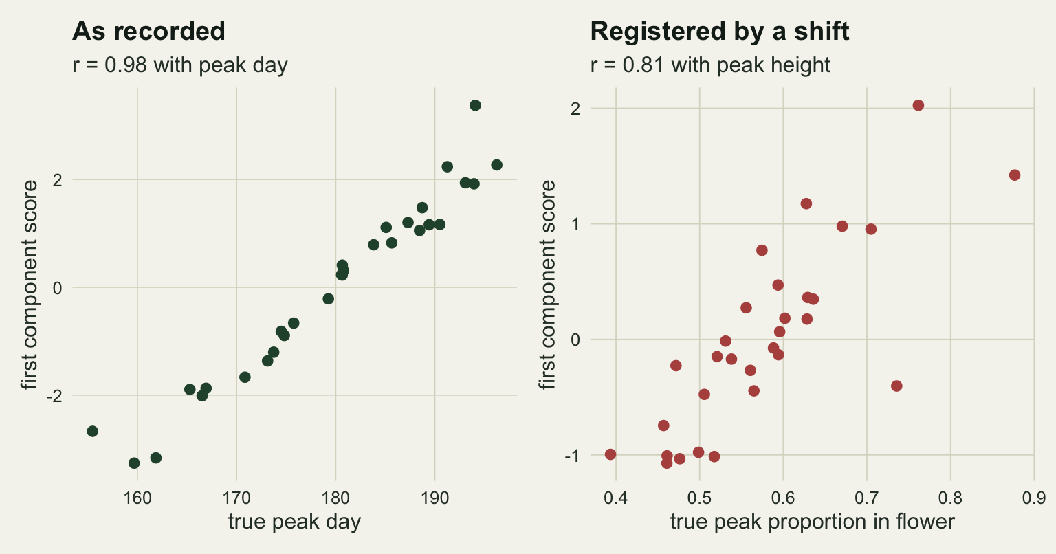
Many sets of seasons, and noisier ones
One set of thirty curves is one draw, and a share of variance from thirty curves has a wide sampling distribution. The pipeline was repeated on two hundred independent sets of seasons with the design above, and then on a hundred sets at each of four noise levels. The replication counts were fixed before running; the time budget for the post set them, not the results. Each set also gets a third registration that no real analysis can have: a shift by the true peak day, which separates the error of the estimated landmark from everything else.
pipeline_stats <- function(s) {
  fit <- smooth_seasons(s$obs)
  wp  <- register_peak(fit)
  shc <- shift_peak(fit, wp$pk_hat)
  orc <- shift_peak(fit, s$peak)
  # common support: grid days that every shifted curve covers without the edge rule
  shv <- wp$pk_hat - mean(wp$pk_hat)
  cs  <- grid_day + min(shv) >= day_lo & grid_day + max(shv) <= day_hi
  pu  <- prcomp(fit)
  pw  <- prcomp(wp$reg)
  ps  <- prcomp(shc)
  mu  <- colMeans(fit)
  su  <- c(diff(mu), NA)
  vu  <- sum(apply(fit, 2, var))
  c(loss_un  = 100 * (1 - max(mu) / mean(apply(fit, 1, max))),
    bias_sh  = 100 * (max(colMeans(shc)) / mean(s$amp) - 1),
    frac_hi  = mean(apply(fit, 1, max) > max(mu)),
    sh_un    = 100 * share_of(pu),
    sh_sh    = 100 * share_of(ps),
    sh_wp    = 100 * share_of(pw),
    sh_or    = 100 * share_of(prcomp(orc)),
    slope_un = abs(cor(pu$rotation[ok_idx, 1], su[ok_idx])),
    amp_sh   = abs(cor(ps$x[, 1], s$amp)),
    amp_wp   = abs(cor(pw$x[, 1], s$amp)),
    leak_sh  = abs(cor(ps$x[, 1], s$peak)),
    leak_wp  = abs(cor(pw$x[, 1], s$peak)),
    pk_err   = sd(wp$pk_hat - s$peak),
    left_sh  = 100 * sum(apply(shc, 2, var)) / vu,
    left_wp  = 100 * sum(apply(wp$reg, 2, var)) / vu,
    sh_un_cs = 100 * share_of(prcomp(fit[, cs])),
    sh_sh_cs = 100 * share_of(prcomp(shc[, cs])),
    cs_drop  = (length(grid_day) - sum(cs)) * 0.5,
    edge     = max(abs(fit[, c(1, length(grid_day))])))
}

n_rep <- 200
set.seed(8830)
rep_tab  <- replicate(n_rep, pipeline_stats(sim_seasons()))
rep_mean <- rowMeans(rep_tab)
rep_se   <- apply(rep_tab, 1, sd) / sqrt(n_rep)
rep_q    <- apply(rep_tab, 1, quantile, probs = c(0.05, 0.95))
p_rate   <- function(hit) c(p = mean(hit), se = sqrt(mean(hit) * (1 - mean(hit)) / length(hit)))
gt_sh    <- p_rate(rep_tab["sh_sh", ] > rep_tab["sh_un", ])
gt_wp    <- p_rate(rep_tab["sh_wp", ] > rep_tab["sh_un", ])
sh_gt_wp <- mean(rep_tab["sh_sh", ] > rep_tab["sh_wp", ])
all_hi   <- mean(rep_tab["frac_hi", ] == 1)
# mean absolute correlation of two independent variables for n = 30
null_abs_r <- sqrt(2 / (pi * (n_curve - 1)))
Across the 200 sets the pointwise mean loses 22.2 per cent of the average peak (Monte Carlo standard error 0.31; 90 per cent of sets between 15.6 and 29.2). The mean curve peaks below every one of the thirty seasons in only 2.5 per cent of sets; on average 86.7 per cent of seasons peak above it, so a handful of low seasons almost always sit under it. The shift-registered mean peak is 1.33 per cent below the true mean height (standard error 0.04).
The shares now separate by warp. The first component explains 61.8 per cent before registration, 74.2 per cent after the shift and 61.0 per cent after the pinned warp (standard errors 0.40, 0.45 and 0.54). The shift raises the share in 91.5 per cent of sets (standard error 2.0), the pinned warp in 46.0 per cent (standard error 3.5), and the shift share beats the warp share in 100.0 per cent of sets. The shift by the true peak day gives 77.0 per cent, so estimating the landmark costs 2.8 percentage points. The single set above, where the shift lowered the share, is one of the minority.
The leak is also clear in the replicates. The absolute correlation of the registered first score with the true peak day averages 0.146 after the shift and 0.232 after the pinned warp (standard errors 0.007 and 0.012). For two unrelated variables and thirty seasons the expected absolute correlation is 0.148, so in this run the shift leaves no detectable timing in the first score and the warp leaves a clear amount. Both first scores track peak height about equally, at 0.896 and 0.882. The unregistered first loading correlates at 0.959 in absolute value with the slope of the mean. Of the pointwise variance, 23.8 per cent survives the shift and 29.6 per cent survives the warp.
noise_grid <- c(0.03, 0.06, 0.10, 0.15)
n_rep_noise <- 100
set.seed(5512)
noise_tab <- do.call(rbind, lapply(noise_grid, function(ns) {
  m_out <- replicate(n_rep_noise, pipeline_stats(sim_seasons(noise = ns)))
  data.frame(noise = ns,
             stat = c(rownames(m_out), "gt_sh", "gt_sh_cs"),
             mean = c(rowMeans(m_out), mean(m_out["sh_sh", ] > m_out["sh_un", ]),
                      mean(m_out["sh_sh_cs", ] > m_out["sh_un_cs", ])),
             se = c(apply(m_out, 1, sd) / sqrt(n_rep_noise), NA, NA))
}))
nget <- function(ns, st, col = "mean") noise_tab[noise_tab$noise == ns & noise_tab$stat == st, col]
noise_lo <- min(noise_grid)
noise_hi <- max(noise_grid)
noise_mid <- noise_grid[3]
# the lowest noise level repeats the design of the two hundred sets: how far apart are the runs?
z_runs <- function(st) (nget(noise_lo, st) - rep_mean[st]) /
  sqrt(nget(noise_lo, st, "se")^2 + rep_se[st]^2)
z_leak_sh <- z_runs("leak_sh")
z_leak_wp <- z_runs("leak_wp")
# shift minus as recorded share, full grid and common support
gap_full <- function(ns) nget(ns, "sh_sh") - nget(ns, "sh_un")
gap_cs   <- function(ns) nget(ns, "sh_sh_cs") - nget(ns, "sh_un_cs")
# does the warp leak change with noise beyond MC error? lowest against highest level
z_wp_lohi <- (nget(noise_lo, "leak_wp") - nget(noise_hi, "leak_wp")) /
  sqrt(nget(noise_lo, "leak_wp", "se")^2 + nget(noise_hi, "leak_wp", "se")^2)
Noise, together with the edge rule of the shift, decides whether the shift raises the share; neither changes the sign for the warp. The peak day error grows from 1.14 days at a noise standard deviation of 0.03 to 3.38 days at 0.15, and the shift-registered first score tracks peak height at 0.882 and 0.819. The shares move far more. On the full grid, after the shift the first component explains 73.2 per cent at the lowest noise and 39.6 per cent at the highest; before registration the figures are 63.2 and 49.6; after the pinned warp 60.2 and 38.5. The shift raises the share in 83 per cent of sets at the lowest noise, 62 per cent at 0.06, and only 25 and 14 per cent at 0.10 and 0.15. On average the pinned warp share is below the unregistered one at every noise level tried.
Part of that reversal belongs to the shift rule rather than to registration. A shifted curve needs values beyond the observation window, and shift_peak() holds it at its end value there. At the design noise the smoothed ends are small: the largest end value per set averages 0.063. At noise 0.15 it averages 0.295, and a noisy end value copied along the edge of the grid is between-curve variance that neither a timing nor a height mode describes. Restricting both matrices to the grid days that every shifted curve covers without the rule (on average 50.4 days fewer at the highest noise) changes the picture at the two higher noise levels. At 0.10 the shift share is 59.0 per cent against 59.7 as recorded (standard errors 0.85 and 0.58), and the shift raises it in 51 per cent of sets, so the two are level. At 0.15 the shift share is still lower, 49.6 against 54.5 per cent, raised in 32 per cent of sets. The gap between the shift and the unregistered share goes from -6.8 to -0.7 points at 0.10 and from -10.0 to -5.0 points at 0.15: the edge rule accounts for most of the reversal at 0.10 and about half of it at 0.15. At the lowest noise the restriction moves the shift share only from 73.2 to 75.5 per cent.
What remains at the highest noise is not landmark error: on the full grid the shift by the true peak day gives 40.5 per cent, close to the estimated shift. A likely reason for the remainder, not separated out here, is that registration removes structured timing variance while the smoothing error left in each curve is spread over many components, so the noisier the curves, the larger the part of what remains that no single component can hold.
The timing leak of the warp shows no clear trend with noise: its mean absolute correlation with the true peak day is 0.300 at the lowest noise and 0.245 at the highest, a difference of 2.1 standard errors, and well above the chance value at every level. For the shift the figures are 0.182 and 0.141, near the chance value at the three higher noise levels and above it at the lowest. The lowest level repeats the design of the two hundred sets above, and the two runs disagree there by 2.7 standard errors for the shift and 3.1 for the warp. The code and design are identical, so that gap is Monte Carlo scatter, somewhat larger than the standard errors suggest, and the lowest-noise leak values should not be read as a rise. What holds in both runs and at every level is the ordering: the shift leak is well under the warp’s.
arm_lab <- c("as recorded", "shift", "pinned warp")
arm_col <- setNames(c(te_ink, te_forest, te_rust), arm_lab)
arm_df <- function(stats, labs) do.call(rbind, lapply(seq_along(stats), function(k)
  data.frame(noise = noise_grid,
             value = sapply(noise_grid, nget, st = stats[k]),
             se = sapply(noise_grid, nget, st = stats[k], col = "se"),
             what = factor(labs[k], levels = arm_lab))))
share_df <- arm_df(c("sh_un", "sh_sh", "sh_wp"), arm_lab)
leak_df  <- arm_df(c("leak_sh", "leak_wp"), arm_lab[2:3])

p_share <- ggplot(share_df, aes(noise, value, colour = what)) +
  geom_line(linewidth = 0.9) +
  geom_errorbar(aes(ymin = value - 1.96 * se, ymax = value + 1.96 * se),
                width = 0.004, linewidth = 0.5) +
  geom_point(size = 2.2) +
  scale_colour_manual(values = arm_col, name = NULL, drop = FALSE) +
  labs(x = "observation noise sd", y = "first component share (per cent)",
       title = "Variance share") +
  theme_datasheet() +
  theme(legend.position = "bottom")
p_leak <- ggplot(leak_df, aes(noise, value, colour = what)) +
  geom_hline(yintercept = null_abs_r, linetype = "dashed", colour = te_body,
             linewidth = 0.5) +
  geom_line(linewidth = 0.9) +
  geom_errorbar(aes(ymin = value - 1.96 * se, ymax = value + 1.96 * se),
                width = 0.004, linewidth = 0.5) +
  geom_point(size = 2.2) +
  scale_colour_manual(values = arm_col, name = NULL, drop = FALSE) +
  coord_cartesian(ylim = c(0, NA)) +
  labs(x = "observation noise sd",
       y = "mean |r| of first score with true peak day",
       title = "Timing leak") +
  theme_datasheet() +
  theme(legend.position = "bottom")
p_share + p_leak + plot_layout(guides = "collect") &
  theme(legend.position = "bottom",
        plot.background = element_rect(fill = te_paper, colour = NA))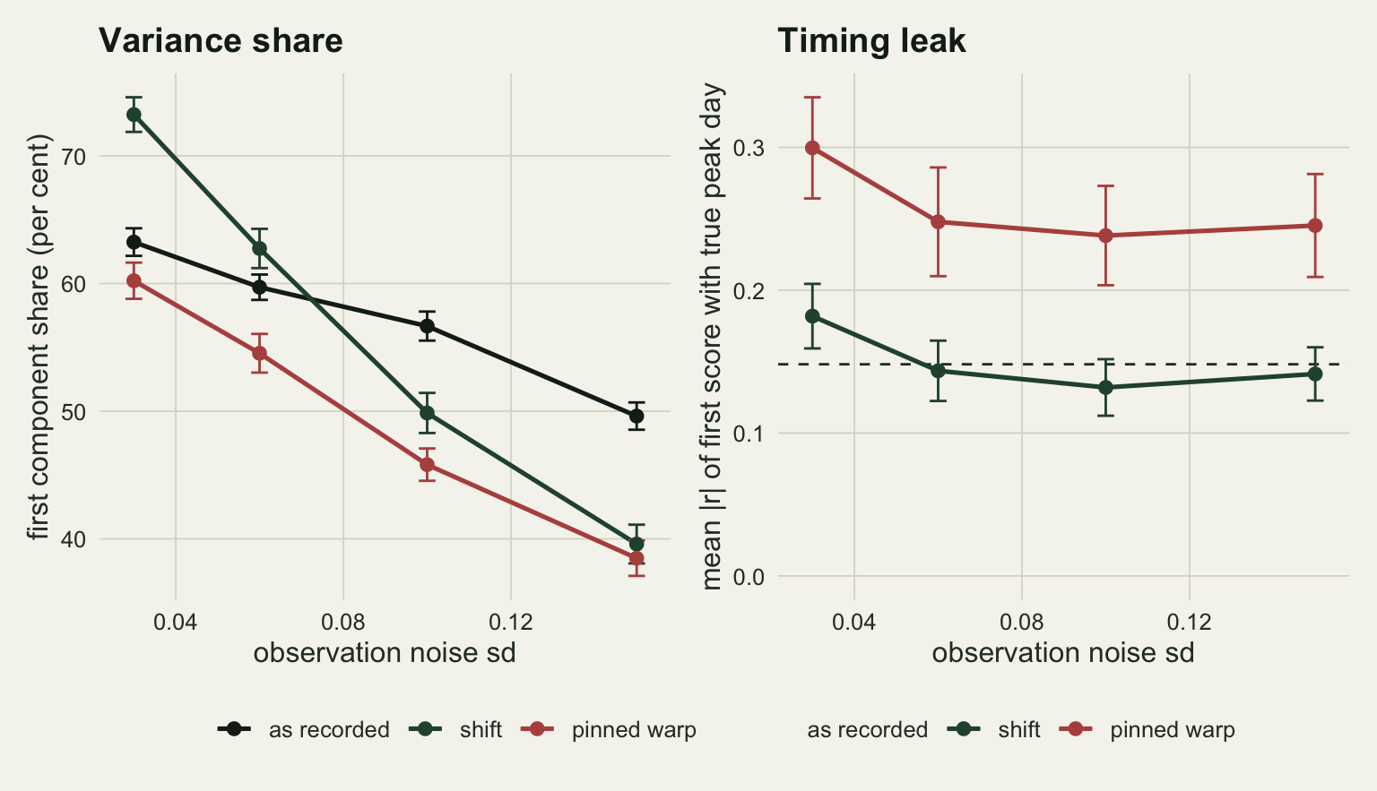
What to report
Report the registration step as part of the method, with the landmark named and the warp family described, and keep the warp. The estimated peak days are a result in their own right: they are the phase variable, and they belong in the same kind of analysis as any other phenological date. Registration moves timing out of the curves; it should not move it out of the paper.
Choose the warp family for the kind of timing variation expected, and say why. Here the seasons differ by translation, and the shift is the family that matches; the pinned piecewise linear warp compressed one limb and stretched the other in proportion to how far each peak had moved, and left timing in the component that was supposed to be free of it. If seasons are thought to differ in duration as well as position, a warp with more landmarks may be the better candidate, but then the same check applies: correlate the registered scores with the estimated peak days, and treat a correlation well beyond chance as timing that the warp has put back.
Report the pointwise mean of unregistered curves only with a warning attached, and never read a peak height or a season width off it. On the design here it took 22.2 per cent off the average peak. The registered mean, drawn on a reference time axis, is the curve to show when the question is what a typical season looks like.
Describe each functional principal component by its shape, and check that shape before interpreting the scores. Whether the share of the first component rises after registration depends on the warp and on the noise: on this design and on the full grid the shift raised it on average at the two lowest noise levels and lowered it at the two highest. On the days that every shifted curve covers, it was level with the unregistered share at a noise standard deviation of 0.10 and lower only at 0.15. The pinned warp lowered it on average at every noise level, if only slightly at the lowest noise, where it still raised the share in 46.0 per cent of two hundred sets. A share that goes up or down is therefore not evidence that registration worked. A first component that looks like minus the slope of the mean curve is a timing mode, whatever its share, and a plot of the loading against the mean curve and against its slope, as in the figure above, costs two lines.
State how much of the between-curve variance registration removed, and give the warp family, the landmarks and the noise level with it. The ratio of summed pointwise variance after and before registration is a single number, but it is not a property of the curves alone: on this design the shift removed 76.2 per cent of the variance and the pinned warp 70.4 per cent.
Honest limits
The seasons here all have exactly one peak, and the peak is a good landmark because it is sharp relative to the noise. A season with two flushes, a flat top, or a truncated start has no single landmark, and picking the highest point then registers some curves on the wrong feature. That produces sharp artefacts in the registered mean and a component that encodes which peak was chosen. Continuous registration, which aligns whole curves to a template by optimising a fit criterion as Ramsay and Li describe, avoids hand-picked landmarks but has its own tuning and can overfit the warp.
The comparison favours the shift because the simulation generates timing as a pure translation. Had the seasons been generated by stretching a template piecewise linearly between the window ends, with only the peak day varying, the pinned warp would be the correct family and the shift the misspecified one. Neither warp aligns width: the width variation in the simulation survives both registrations on purpose. How much variation to call phase and how much to call amplitude is a modelling choice, not something the data decide; Marron and colleagues discuss that ambiguity and the alternative frameworks for it at length. The shift also needs a rule at the window edges; here the curve is held at its end value. In the first set that is harmless, because no smoothed season is further than 0.054 from zero at either end of the window, but at high noise the ends of the smoothed curves wander, and the held values account for most of the fall of the shift share below the unregistered one at a noise standard deviation of 0.10 and about half of it at 0.15. Comparing shares only on the days every shifted curve covers avoids the rule, at the cost of about 50 days of the window at the design noise.
The simulation uses a known shape family, a two-sided Gaussian, with timing, height and width varied independently. Real seasons couple them: late seasons are often shorter and lower. With that coupling, even a correct registration leaves timing information in the first score through its correlation with height, and the leak of a misspecified warp adds to that. The separation measured for the shift should be read as a best case.
Smoothing was done once per curve with generalised cross-validation, and the smoothing error was ignored downstream. The principal components were computed as if the smoothed curves were exact. That is standard practice, but how much of each component is smoothing error was not separated out here, and no uncertainty for loadings or scores is given. A bootstrap over seasons would be the next step.
The whole analysis runs on thirty curves on a regular half-day grid. Irregular or sparse sampling, with a few visits per season at different days, calls for the sparse functional data methods that pool information across curves when estimating each one, and the per-curve smoothing used here would break down.
References
Kneip A, Gasser T 1992 The Annals of Statistics 20(3):1266-1305 (10.1214/aos/1176348769)
Ramsay JO, Silverman BW 2005 Functional Data Analysis, 2nd edition (ISBN 978-0-387-40080-8)
Ramsay JO, Li X 1998 Journal of the Royal Statistical Society Series B 60(2):351-363 (10.1111/1467-9868.00129)
Marron JS, Ramsay JO, Sangalli LM, Srivastava A 2015 Statistical Science 30(4):468-484 (10.1214/15-STS524)