Harmonics or cyclic splines for a narrow seasonal peak

Cyclic splines in mgcv for a narrow seasonal peak in counts: harmonics chosen by AIC or BIC against s(day, bs = ‘cc’), and the New Year jump of a plain smooth.

A light trap on the edge of an oak wood is run one night a week, all year. For most of the year it catches almost nothing of one geometrid, and then for a few weeks around the middle of December it catches it every time. A flight period like that is the shape a lot of phenological data takes: a flowering pulse, a hatch, the passage of a migrant through a ringing site. The analyst wants two things from a year of counts, the date of the peak and how long the flight period lasts, and wants them from a smooth curve rather than from the single highest night.

The question for this post is which smooth curve. Harmonic regression on a seasonal raster fitted sines and cosines to a canopy greenness series and found that two harmonics gave the best peak day, and it said plainly that the recommendation was conditional on the shape: one broad season with a moderately asymmetric crest. A pulse a few weeks wide is the shape it warned about, since a narrow bump needs many harmonics, and the number of harmonics then has to be chosen from the data. The alternative is a penalised spline that is forced to join itself at the end of the year, s(day, bs = "cc") in mgcv, which lets REML choose the wiggliness instead. Placing this pulse in December is deliberate. Phenology in R: day of year and event timing shows the arithmetic mean of dates on either side of New Year landing in midsummer, and circular data and the von Mises distribution opens with the same trap for bearings; a regression smooth on day of year has its own version of it.

The expectation going in was that the cyclic spline would recover the width and date of a narrow peak better than harmonics chosen by an information criterion. Measured over simulated seasons, that expectation failed for the cyclic spline as mgcv fits it by default. Harmonics chosen by AIC gave the least widened narrow pulse at every count level tried; the cyclic spline with REML was close to them when counts were high and nearly as wide as the BIC choice when counts were low. The widening turned out to belong to REML’s choice of smoothing parameter, not to the spline: the same basis with mgcv’s UBRE criterion kept the pulse about as narrow as AIC did, at the price of an occasional runaway crest. Every fit put the peak a few days late on average. What the cyclic spline does settle is the year boundary, and there the measurement is unambiguous, including for the cyclic spline itself when its end knots are left at their defaults.

library(ggplot2)
library(mgcv)

te_paper  <- "#f5f4ee"
te_ink    <- "#16241d"
te_body   <- "#2c3a31"
te_forest <- "#275139"
te_rust   <- "#b5534e"
te_gold   <- "#c9b458"
te_line   <- "#dad9ca"

theme_datasheet <- function() {
  theme_minimal(base_size = 12) +
    theme(plot.background  = element_rect(fill = te_paper, colour = NA),
          panel.background = element_rect(fill = te_paper, colour = NA),
          panel.grid.major = element_line(colour = te_line, linewidth = 0.3),
          panel.grid.minor = element_blank(),
          text             = element_text(colour = te_body),
          plot.title       = element_text(colour = te_ink, face = "bold"),
          plot.subtitle    = element_text(colour = te_body),
          axis.text        = element_text(colour = te_body))
}

A flight period a few weeks wide

The simulated trap is run on day 3 of the year and every seventh day after it, so a year holds 52 trap nights. The expected catch is a background of half a moth per night plus a pulse peaking on day 350, the middle of December. The pulse rises faster than it falls, with a standard deviation of 6 days before the peak and 12 days after it, because flight periods usually build quickly and tail off as the last individuals die. The pulse is wrapped around the year so that its tail runs into January. Counts are Poisson. Every design constant below was fixed before the first replicate was run.

Width is measured the same way for the truth and for every fitted curve: on a grid of quarter days, take the curve’s minimum as its background, and count the days on which the curve stands more than half-way from that background to its maximum, following the run of such days outwards from the maximum and around the year if necessary. The peak date is the grid day of the maximum, and date errors are taken around the circle.

year_len  <- 365
visit_day <- seq(3, 365, by = 7)
n_visit   <- length(visit_day)
peak_day  <- 350
rise_sd   <- 6
fall_sd   <- 12
base_rate <- 0.5
k_max     <- 8
k_cc      <- 30
day_fine  <- seq(0.5, 365.5, by = 0.25)

circ_gap <- function(d) ((d + year_len / 2) %% year_len) - year_len / 2

pulse_mean <- function(d, peak, s_rise, s_fall, base, height) {
  bump <- 0
  for (m in -2:2) {
    z <- d - peak + year_len * m
    bump <- bump + exp(-z^2 / (2 * ifelse(z < 0, s_rise, s_fall)^2))
  }
  base + height * bump
}

harm_design <- function(d, n_harm) {
  w <- 2 * pi * d / year_len
  X <- matrix(1, length(d), 1 + 2 * n_harm)
  for (k in seq_len(n_harm)) {
    X[, 2 * k] <- cos(k * w)
    X[, 2 * k + 1] <- sin(k * w)
  }
  X
}

half_max <- function(f) {
  f_base <- min(f)
  i_top  <- which.max(f)
  above  <- rep(f > f_base + (max(f) - f_base) / 2, 3)
  n_f <- length(f)
  lo <- i_top + n_f
  hi <- lo
  while (lo > 1 && above[lo - 1]) lo <- lo - 1
  while (hi < 3 * n_f && above[hi + 1]) hi <- hi + 1
  c(peak = day_fine[i_top], width = min(hi - lo + 1, n_f) * 0.25)
}

truth_narrow <- half_max(pulse_mean(day_fine, peak_day, rise_sd, fall_sd,
                                    base_rate, 10))
truth_narrow

  peak  width 
350.00  21.25 

With a pulse height of 10 moths per night, the true half-maximum width is 21.25 days. Two sampling facts follow from the design. Weekly visits put about three trap nights inside that window, and the nights either side of the peak fall on days 346 and 353, neither of them on the peak.

Before adding noise it helps to see how much of the problem is the curve family rather than the counts. The next chunk fits the exact expected catch on the 52 trap nights, with no Poisson noise at all, once with eight harmonics and once with a cyclic spline that has a larger basis and almost no penalty.

exact_mu <- pulse_mean(visit_day, peak_day, rise_sd, fall_sd, base_rate, 10)
exact_h8 <- suppressWarnings(glm.fit(harm_design(visit_day, k_max), exact_mu,
                                     family = poisson()))$coefficients
exact_h8_fit <- half_max(exp(drop(harm_design(day_fine, k_max) %*% exact_h8)))
exact_cc <- suppressWarnings(gam(exact_mu ~ s(visit_day, bs = "cc", k = 45),
                                 family = quasipoisson, sp = 1e-6,
                                 knots = list(visit_day = c(0.5, 365.5))))
exact_cc_fit <- half_max(predict(exact_cc, data.frame(visit_day = day_fine),
                                 type = "response"))
rbind(truth = truth_narrow, harmonics_8 = exact_h8_fit, cyclic_unpenalised = exact_cc_fit)

                     peak width
truth              350.00 21.25
harmonics_8        353.75 20.50
cyclic_unpenalised 350.75 22.25

Eight harmonics put the peak 3.75 days late with a width of 20.50 days, and the nearly unpenalised cyclic spline puts it 0.75 days late with a width of 22.25 days. An eight-term Fourier series cannot follow a lopsided pulse exactly, and its crest leans towards the long tail. That offset is a property of truncation, the same for every season, and it is the reference line for the rest of the post, not its result. The questions that need a simulation are what happens when the number of harmonics is chosen from noisy counts, and what REML does with the same counts.

Harmonics chosen by AIC and BIC against a cyclic spline

The harmonic model is a Poisson GLM on the log scale with an intercept and K pairs of sine and cosine terms at 1, 2, … K cycles per year, the form Stolwijk, Straatman and Zielhuis set out for seasonality in regression. K runs from 1 to 8 and is chosen separately in each season, once by AIC and once by BIC (Schwarz 1978), from the Poisson log-likelihood.

The cyclic spline is a cubic regression spline whose value and first two derivatives are forced to match at its two end knots. In mgcv the end knots are, by default, the smallest and largest values of the covariate in the data. For day of year that is not the year: here it would join day 3 to day 360 as though they were the same instant. The knots = list(day = c(0.5, 365.5)) argument puts the ends a full year apart, half a day beyond the first and the last day of the year, so the curve on 31 December runs straight into the curve on 1 January. Wood’s book gives the construction; the basis dimension is k = 30 and the smoothing parameter is chosen by REML (Wood 2011), mgcv’s recommended default. In the replicate study the same smooth is also fitted with method = "GCV.Cp", which for a Poisson family is UBRE, an AIC-like prediction criterion, because the choice of criterion turns out to matter for a narrow crest.

fit_harmonics <- function(day, y) {
  n_obs <- length(y)
  fits <- lapply(seq_len(k_max), function(K) {
    X <- harm_design(day, K)
    gf <- suppressWarnings(glm.fit(X, y, family = poisson()))
    list(cf = gf$coefficients, npar = ncol(X),
         loglik = sum(dpois(y, gf$fitted.values, log = TRUE)))
  })
  loglik <- sapply(fits, `[[`, "loglik")
  npar   <- sapply(fits, `[[`, "npar")
  k_aic <- which.min(-2 * loglik + 2 * npar)
  k_bic <- which.min(-2 * loglik + log(n_obs) * npar)
  list(k_aic = k_aic, k_bic = k_bic,
       aic = exp(drop(harm_design(day_fine, k_aic) %*% fits[[k_aic]]$cf)),
       bic = exp(drop(harm_design(day_fine, k_bic) %*% fits[[k_bic]]$cf)))
}

fit_cyclic <- function(day, y, k_basis = k_cc, crit = "REML") {
  gam(y ~ s(day, bs = "cc", k = k_basis), family = poisson,
      method = crit, knots = list(day = c(0.5, 365.5)))
}

set.seed(3504)
one_mu <- pulse_mean(visit_day, peak_day, rise_sd, fall_sd, base_rate, 10)
one_y  <- rpois(n_visit, one_mu)
one_h  <- fit_harmonics(visit_day, one_y)
one_cc <- fit_cyclic(visit_day, one_y)
one_cc_curve <- predict(one_cc, data.frame(day = day_fine), type = "response")
one_tab <- rbind(truth = truth_narrow, aic = half_max(one_h$aic),
                 bic = half_max(one_h$bic), cyclic = half_max(one_cc_curve))
one_tab

        peak width
truth  350.0 21.25
aic    355.0 26.00
bic    356.0 37.25
cyclic 355.5 25.50

c(k_aic = one_h$k_aic, k_bic = one_h$k_bic, edf = sum(one_cc$edf) - 1)

   k_aic    k_bic      edf 
5.000000 3.000000 8.370911 

top_idx <- order(one_y, decreasing = TRUE)[1:2]
rbind(day = visit_day[top_idx], count = one_y[top_idx])

      [,1] [,2]
day    353  360
count   14   13

In this one season AIC chose 5 harmonics and BIC chose 3, and the REML cyclic spline used 8.4 effective degrees of freedom. Against a true width of 21.25 days, the widths came out at 26.00 days for the AIC choice, 25.50 for the cyclic spline and 37.25 for the BIC choice. All three put the peak between 5.0 and 6.0 days late. One season decides nothing, but the figure shows what the numbers are measuring.

shift_day <- function(d) (d - 182) %% year_len
month_at  <- shift_day(c(182, 244, 305, 1, 60, 121))
month_lab <- c("1 Jul", "1 Sep", "1 Nov", "1 Jan", "1 Mar", "1 May")
curve_df <- rbind(
  data.frame(day = day_fine, rate = pulse_mean(day_fine, peak_day, rise_sd,
             fall_sd, base_rate, 10), fit = "true mean"),
  data.frame(day = day_fine, rate = one_h$aic,
             fit = sprintf("harmonics, AIC (%d)", one_h$k_aic)),
  data.frame(day = day_fine, rate = one_h$bic,
             fit = sprintf("harmonics, BIC (%d)", one_h$k_bic)),
  data.frame(day = day_fine, rate = one_cc_curve, fit = "cyclic spline, REML"))
curve_df$pos <- shift_day(curve_df$day)
curve_df <- curve_df[order(curve_df$fit, curve_df$pos), ]
curve_df$fit <- factor(curve_df$fit, levels = c("true mean",
  sprintf("harmonics, AIC (%d)", one_h$k_aic),
  sprintf("harmonics, BIC (%d)", one_h$k_bic), "cyclic spline, REML"))
fit_cols <- setNames(c(te_line, te_gold, te_rust, te_forest), levels(curve_df$fit))
pts_df <- data.frame(pos = shift_day(visit_day), count = one_y)

ggplot() +
  geom_line(data = curve_df, aes(pos, rate, colour = fit,
                                 linewidth = fit == "true mean")) +
  geom_point(data = pts_df, aes(pos, count), colour = te_ink, size = 1.6) +
  scale_linewidth_manual(values = c(0.8, 2.2), guide = "none") +
  scale_colour_manual(values = fit_cols, name = NULL) +
  scale_x_continuous(breaks = month_at, labels = month_lab) +
  coord_cartesian(xlim = shift_day(c(305, 60))) +
  labs(x = NULL, y = "moths per trap night",
       title = "One season, three smoothers",
       subtitle = "weekly trap nights; the peak sits in mid December") +
  guides(colour = guide_legend(nrow = 2)) +
  theme_datasheet() +
  theme(legend.position = "bottom")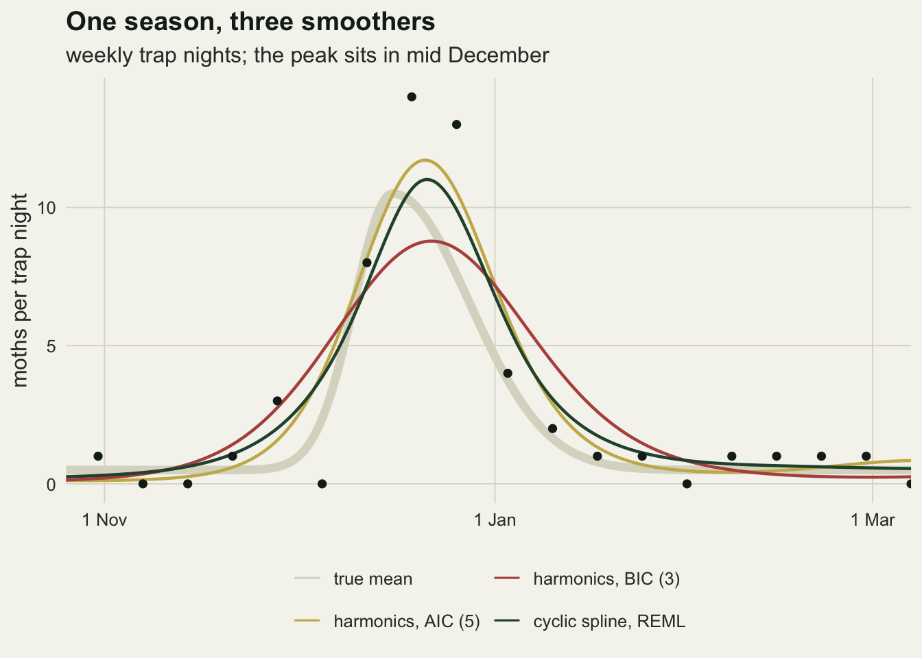

Figure 1: One simulated season of weekly light-trap counts, shown from November to early March so that the December pulse is not split by the calendar. The broad pale line is the true mean; the three fitted curves are harmonics chosen by AIC, harmonics chosen by BIC and a cyclic spline fitted by REML, with the selected number of harmonics in the legend.

The two highest counts, 14 and 13 moths, fell on days 353 and 360, the first two trap nights after the true crest, while the night of day 346 caught 8. The fitted curves follow those counts, which is why all three crests sit to the right of the true one in this season.

Three hundred seasons

Four scenarios repeat that season 300 times each. Three keep the narrow pulse and change its height to 20, 10 and 4 moths per night, which is the noise level: at a height of 4 the peak nights hold a handful of moths. The fourth is a control with a broad season, standard deviations of 30 and 50 days, close to the kind of curve the harmonic regression post worked with. In every replicate the harmonic count is chosen afresh by AIC and by BIC, and the cyclic spline is refitted twice to the same counts, once with REML and once with UBRE.

one_season <- function(s_rise, s_fall, height) {
  y  <- rpois(n_visit, pulse_mean(visit_day, peak_day, s_rise, s_fall,
                                  base_rate, height))
  hf <- fit_harmonics(visit_day, y)
  warned <- c(reml = FALSE, ubre = FALSE)
  flag <- function(expr, which_fit) withCallingHandlers(expr, warning = function(w) {
    warned[[which_fit]] <<- TRUE
    invokeRestart("muffleWarning")
  })
  fit_re <- flag(fit_cyclic(visit_day, y), "reml")
  fit_ub <- flag(fit_cyclic(visit_day, y, crit = "GCV.Cp"), "ubre")
  cc <- predict(fit_re, data.frame(day = day_fine), type = "response")
  ub <- predict(fit_ub, data.frame(day = day_fine), type = "response")
  mu_true <- pulse_mean(day_fine, peak_day, s_rise, s_fall, base_rate, height)
  tr <- half_max(mu_true)
  est <- rbind(half_max(hf$aic), half_max(hf$bic), half_max(cc), half_max(ub))
  c(k_aic = hf$k_aic, k_bic = hf$k_bic,
    peak_err = circ_gap(est[, "peak"] - tr["peak"]),
    width_ratio = est[, "width"] / tr["width"],
    sq_err = sapply(list(hf$aic, hf$bic, cc, ub), function(f) mean((f - mu_true)^2)),
    top_ratio = sapply(list(hf$aic, hf$bic, cc, ub), max) / max(mu_true),
    edf_reml = sum(fit_re$edf) - 1, edf_ubre = sum(fit_ub$edf) - 1,
    warn_reml = warned[["reml"]], warn_ubre = warned[["ubre"]])
}

scen_tab <- data.frame(
  scenario = c("narrow, peak 20", "narrow, peak 10", "narrow, peak 4",
               "broad, peak 10"),
  s_rise = c(rise_sd, rise_sd, rise_sd, 30),
  s_fall = c(fall_sd, fall_sd, fall_sd, 50),
  height = c(20, 10, 4, 10))
n_rep <- 300

set.seed(8126)
rep_out <- lapply(seq_len(nrow(scen_tab)), function(i)
  t(replicate(n_rep, one_season(scen_tab$s_rise[i], scen_tab$s_fall[i],
                                scen_tab$height[i]))))
colnames(rep_out[[1]])

 [1] "k_aic"        "k_bic"        "peak_err1"    "peak_err2"    "peak_err3"   
 [6] "peak_err4"    "width_ratio1" "width_ratio2" "width_ratio3" "width_ratio4"
[11] "sq_err1"      "sq_err2"      "sq_err3"      "sq_err4"      "top_ratio1"  
[16] "top_ratio2"   "top_ratio3"   "top_ratio4"   "edf_reml"     "edf_ubre"    
[21] "warn_reml"    "warn_ubre"   

method_lab <- c("harmonics, AIC", "harmonics, BIC", "cyclic spline, REML",
                "cyclic spline, UBRE")
summ <- do.call(rbind, lapply(seq_len(nrow(scen_tab)), function(i) {
  r_mat <- rep_out[[i]]
  w_mat <- r_mat[, paste0("width_ratio", 1:4)]
  p_mat <- r_mat[, paste0("peak_err", 1:4)]
  data.frame(scenario = scen_tab$scenario[i], method = method_lab,
             width_med = apply(w_mat, 2, median),
             width_lo = apply(w_mat, 2, quantile, 0.25),
             width_hi = apply(w_mat, 2, quantile, 0.75),
             wide_share = colMeans(w_mat > 1.5),
             wide_se = sqrt(colMeans(w_mat > 1.5) * (1 - colMeans(w_mat > 1.5)) / n_rep),
             peak_bias = colMeans(p_mat),
             peak_se = apply(p_mat, 2, sd) / sqrt(n_rep),
             peak_mae = colMeans(abs(p_mat)),
             peak_far = colMeans(abs(p_mat) > 30),
             sq_err_med = apply(r_mat[, paste0("sq_err", 1:4)], 2, median),
             runaway = colMeans(r_mat[, paste0("top_ratio", 1:4)] > 2))
}))
rownames(summ) <- NULL
print(summ, digits = 3)

          scenario              method width_med width_lo width_hi wide_share
1  narrow, peak 20      harmonics, AIC     1.000    0.906     1.09    0.00667
2  narrow, peak 20      harmonics, BIC     1.094    1.000     1.26    0.03333
3  narrow, peak 20 cyclic spline, REML     1.059    0.976     1.15    0.00333
4  narrow, peak 20 cyclic spline, UBRE     1.018    0.906     1.12    0.00333
5  narrow, peak 10      harmonics, AIC     1.094    0.941     1.31    0.11000
6  narrow, peak 10      harmonics, BIC     1.471    1.221     1.88    0.48000
7  narrow, peak 10 cyclic spline, REML     1.318    1.165     1.51    0.26667
8  narrow, peak 10 cyclic spline, UBRE     1.141    0.985     1.31    0.08667
9   narrow, peak 4      harmonics, AIC     1.541    1.106     2.41    0.52000
10  narrow, peak 4      harmonics, BIC     3.471    2.159     6.76    0.91000
11  narrow, peak 4 cyclic spline, REML     3.100    2.047     5.45    0.94667
12  narrow, peak 4 cyclic spline, UBRE     1.600    1.268     2.30    0.57667
13  broad, peak 10      harmonics, AIC     0.976    0.856     1.08    0.00000
14  broad, peak 10      harmonics, BIC     1.065    0.958     1.11    0.00000
15  broad, peak 10 cyclic spline, REML     0.968    0.897     1.04    0.00000
16  broad, peak 10 cyclic spline, UBRE     0.976    0.901     1.04    0.00000
   wide_se peak_bias peak_se peak_mae peak_far sq_err_med runaway
1  0.00470      3.80  0.1071     3.83  0.00000      0.847 0.00000
2  0.01036      4.40  0.0918     4.41  0.00000      1.025 0.00000
3  0.00333      3.89  0.0795     3.89  0.00000      0.779 0.00000
4  0.00333      3.38  1.5135     8.96  0.05000      0.784 0.04000
5  0.01806      4.33  0.2590     4.41  0.00333      0.501 0.00667
6  0.02884      4.66  0.2648     4.78  0.00333      0.699 0.00333
7  0.02553      4.08  0.1077     4.12  0.00000      0.510 0.00000
8  0.01624      5.47  1.3729     8.80  0.05333      0.458 0.04667
9  0.02884      3.25  1.0179     8.49  0.04000      0.290 0.00667
10 0.01652      6.05  0.9458    11.94  0.08333      0.474 0.00000
11 0.01297      4.70  0.7293     8.09  0.04333      0.362 0.00000
12 0.02853      5.26  1.2616     9.06  0.04667      0.232 0.03000
13 0.00000      9.10  0.5988    11.72  0.02667      0.511 0.00000
14 0.00000     12.69  0.3250    12.96  0.00000      0.478 0.00000
15 0.00000      7.44  0.4450     8.61  0.01000      0.354 0.00000
16 0.00000      7.33  0.6458    10.06  0.01667      0.415 0.00000

paired <- t(sapply(rep_out, function(r_mat) {
  d_log <- log(r_mat[, "width_ratio3"]) - log(r_mat[, "width_ratio1"])
  d_ub <- log(r_mat[, "width_ratio4"]) - log(r_mat[, "width_ratio1"])
  c(mean = mean(d_log), se = sd(d_log) / sqrt(n_rep),
    cc_narrower = mean(r_mat[, "width_ratio3"] < r_mat[, "width_ratio1"]),
    ub_mean = mean(d_ub), ub_se = sd(d_ub) / sqrt(n_rep),
    ub_narrower = mean(r_mat[, "width_ratio4"] < r_mat[, "width_ratio1"]),
    edf_reml = median(r_mat[, "edf_reml"]), edf_ubre = median(r_mat[, "edf_ubre"]),
    warn_reml = mean(r_mat[, "warn_reml"]), warn_ubre = mean(r_mat[, "warn_ubre"]))
}))
paired

           mean          se cc_narrower     ub_mean      ub_se ub_narrower
[1,] 0.05860379 0.006176337   0.2866667 -0.12907992 0.03669451   0.4533333
[2,] 0.18613631 0.011881169   0.1700000 -0.12088986 0.04160617   0.3900000
[3,] 0.61499559 0.036419666   0.1233333 -0.03078474 0.03082025   0.4000000
[4,] 0.00884420 0.006502171   0.4966667 -0.01842016 0.01470043   0.5100000
     edf_reml  edf_ubre warn_reml   warn_ubre
[1,] 9.608839 11.037372         0 0.000000000
[2,] 7.905150 10.094457         0 0.010000000
[3,] 4.010289  7.885457         0 0.003333333
[4,] 4.991323  4.398949         0 0.000000000

pick <- function(s, m, col) summ[summ$scenario == s & summ$method == m, col]
sel_stats <- t(sapply(rep_out, function(r_mat)
  c(aic_mode = which.max(tabulate(r_mat[, "k_aic"], k_max)),
    bic_mode = which.max(tabulate(r_mat[, "k_bic"], k_max)),
    aic_mean = mean(r_mat[, "k_aic"]), bic_mean = mean(r_mat[, "k_bic"]),
    aic_ceiling = mean(r_mat[, "k_aic"] == k_max),
    bic_le3 = mean(r_mat[, "k_bic"] <= 3),
    bic_one = mean(r_mat[, "k_bic"] == 1))))
sel_stats

     aic_mode bic_mode aic_mean bic_mean aic_ceiling   bic_le3     bic_one
[1,]        5        4 5.860000 4.733333 0.136666667 0.0500000 0.000000000
[2,]        5        4 5.553333 3.810000 0.116666667 0.4100000 0.003333333
[3,]        4        1 4.206667 1.926667 0.073333333 0.9033333 0.473333333
[4,]        2        1 2.293333 1.313333 0.003333333 0.9900000 0.723333333

Take the three fits of the original comparison first. At the highest pulse they are close. The median width ratio is 1.00 for the AIC choice, 1.06 for the REML cyclic spline and 1.09 for the BIC choice. As the counts fall they separate. At a height of 10 the medians are 1.09, 1.32 and 1.47, and the share of seasons in which the fitted pulse is more than half as wide again as the truth is 0.110, 0.267 and 0.480 (Monte Carlo standard errors 0.018, 0.026 and 0.029). At a height of 4 the medians are 1.54, 3.10 and 3.47.

The comparison that matters for the original expectation is paired, because the AIC choice and the cyclic spline are fitted to the same counts. On the log scale the REML cyclic spline’s width minus the AIC width averages 0.059 (standard error 0.006) at a height of 20, 0.186 (0.012) at 10 and 0.615 (0.036) at 4: a cyclic pulse wider by 6, 20 and 85 per cent on the geometric mean. The REML fit was the narrower of the two in only 0.287, 0.170 and 0.123 of seasons. In the broad control the difference is 0.009 with a standard error of 0.007, and all four fits have median width ratios between 0.97 and 1.06.

The fourth fit asks whether that loss belongs to the spline or to REML. With the same basis, the same knots and the same counts, UBRE gives median width ratios of 1.02, 1.14 and 1.60 at heights of 20, 10 and 4, against 1.00, 1.09 and 1.54 for AIC, and it is narrower than the AIC fit in 0.453, 0.390 and 0.400 of seasons (a count that includes the runaway fits described below, whose crests are far too narrow). Its share of pulses more than half as wide again as the truth at a height of 10 is 0.087 (standard error 0.016). The median effective degrees of freedom at that height are 7.91 under REML and 10.09 under UBRE, so UBRE simply smooths less. The lighter smoothing has a cost. In 0.047 of seasons at a height of 10 (and 0.040 at 20) the UBRE crest rose to more than twice the true maximum, a runaway spike, against 0.000 for REML; mgcv raised a convergence warning in only 0.010 of the UBRE fits at that height, so the warning misses most of them. On the median squared error of the whole curve, on the rate scale over every quarter day of the year, AIC, REML and UBRE are close and BIC trails, 0.501 for AIC, 0.699 for BIC, 0.510 for REML and 0.458 for UBRE at a height of 10: REML gives up width at the crest without losing much on the curve as a whole.

So the thesis that REML on a cyclic spline recovers a narrow pulse better than a selected harmonic model did not survive, and the comparison that decided it is between smoothing criteria rather than curve families: AIC for the harmonics and UBRE for the spline are both prediction criteria, and they widen the pulse by similar amounts; REML smooths more. The part that did survive is about BIC. Its penalty of log 52 per parameter, 3.95, against 2 for AIC, stops the harmonic series before the pulse is resolved, and at a height of 10 its median width ratio is the largest of the four.

summ$scenario <- factor(summ$scenario, levels = rev(scen_tab$scenario))
summ$method <- factor(summ$method, levels = method_lab)
ggplot(summ, aes(y = scenario, colour = method)) +
  geom_vline(xintercept = 1, linetype = "dashed", colour = te_ink, linewidth = 0.5) +
  geom_linerange(aes(xmin = width_lo, xmax = width_hi),
                 position = position_dodge(width = 0.6), linewidth = 1.1) +
  geom_point(aes(x = width_med), position = position_dodge(width = 0.6), size = 2.6) +
  scale_colour_manual(values = c(te_gold, te_rust, te_forest, "#86a98f"), name = NULL) +
  scale_x_log10(breaks = c(0.75, 1, 1.5, 2, 3, 4, 6),
                labels = c("0.75", "1", "1.5", "2", "3", "4", "6")) +
  labs(x = "fitted half-maximum width / true width (log scale)", y = NULL,
       title = "Which fit widens the pulse",
       subtitle = "median and interquartile range over 300 simulated seasons") +
  guides(colour = guide_legend(reverse = FALSE)) +
  theme_datasheet() +
  theme(legend.position = "bottom")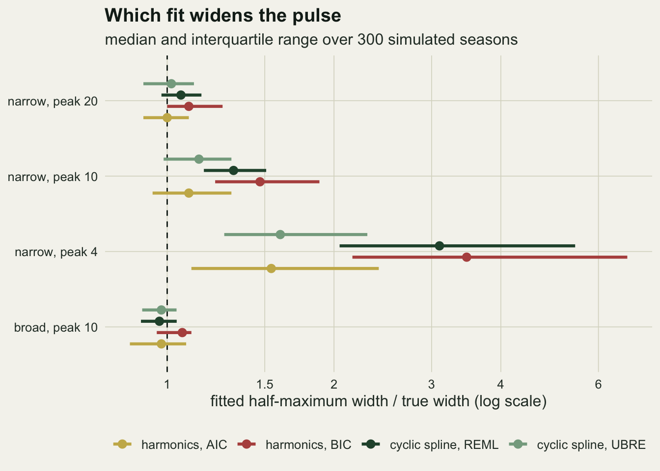

Figure 2: Fitted half-maximum width divided by the true width, over 300 simulated seasons per scenario, for harmonics chosen by AIC, harmonics chosen by BIC and one cyclic spline basis whose smoothing parameter is chosen by REML or by UBRE. Points are medians and bars are interquartile ranges; the dashed line marks a width recovered exactly. Three scenarios have the narrow pulse at peak heights of 20, 10 and 4 moths per night, and the fourth is a broad season.

The selected harmonic counts explain the ordering. At a height of 10, AIC chose 5.55 harmonics on average and BIC 3.81; BIC chose three or fewer in 0.410 of seasons, and at a height of 4 in 0.903. AIC reached the ceiling of 8 in 0.137 of seasons at the highest pulse and 0.073 at the lowest, so the upper limit of the search is binding in a minority of seasons and not in most. In the broad control the most common choice was 2 harmonics by AIC and 1 by BIC, which kept a single harmonic in 0.723 of seasons.

sel_df <- do.call(rbind, lapply(seq_len(nrow(scen_tab)), function(i) {
  r_mat <- rep_out[[i]]
  rbind(data.frame(k = seq_len(k_max), share = tabulate(r_mat[, 1], k_max) / n_rep,
                   rule = "AIC", scenario = scen_tab$scenario[i]),
        data.frame(k = seq_len(k_max), share = tabulate(r_mat[, 2], k_max) / n_rep,
                   rule = "BIC", scenario = scen_tab$scenario[i]))
}))
sel_df$scenario <- factor(sel_df$scenario, levels = scen_tab$scenario)
ggplot(sel_df, aes(k, share, fill = rule)) +
  geom_col(position = position_dodge(width = 0.8), width = 0.75) +
  facet_wrap(~ scenario, nrow = 1) +
  scale_fill_manual(values = c(te_gold, te_rust), name = NULL) +
  scale_x_continuous(breaks = 1:8) +
  labs(x = "harmonics selected (1 to 8)", y = "share of seasons",
       title = "BIC stops earlier, and earlier still when counts are low") +
  theme_datasheet() +
  theme(legend.position = "bottom", strip.text = element_text(colour = te_ink))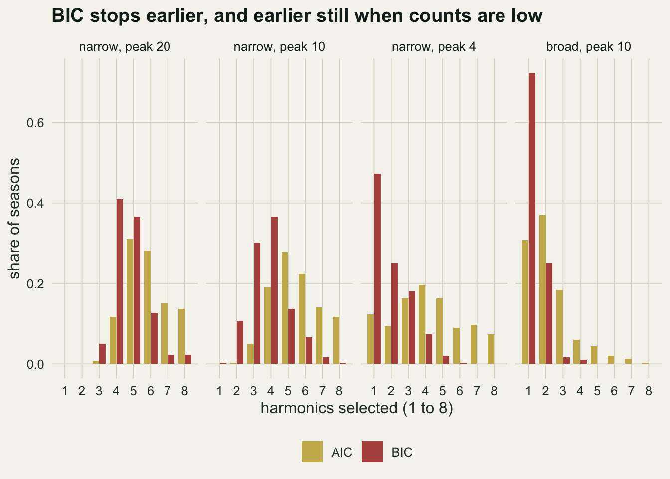

Figure 3: Share of the 300 simulated seasons in each scenario in which AIC and BIC chose each number of harmonics, from 1 to 8.

None of the fits gets the date right, and none of the three original fits gets it much more right than the others. At a height of 10 the mean peak date error is 4.33 days for the AIC choice (Monte Carlo standard error 0.26), 4.08 (0.11) for the REML cyclic spline and 4.66 (0.26) for the BIC choice, all late and all similar in size to the noiseless eight-harmonic offset; for the REML cyclic spline, which was 0.75 days late without noise, the offset is added by the smoothing. The REML cyclic spline’s date errors are the least scattered: at a height of 10 their standard deviation is 1.86 days against 4.49 for AIC and 4.59 for BIC, and at a height of 4 its mean absolute date error is 8.09 days against 8.49 for AIC and 11.94 for BIC. The UBRE fit is the one to watch here: its peak was more than 30 days from the truth in 0.053 of seasons at a height of 10, against 0.000 for REML, and its mean absolute date error there is 8.80 days. In the broad control the offsets are larger: 9.10 days for AIC, 7.44 for REML, 7.33 for UBRE and 12.69 for BIC, the last because BIC mostly keeps a single harmonic, a symmetric curve whose crest sits between the fast rise and the slow fall.

n_check <- 60
set.seed(5530)
k_check <- t(replicate(n_check, {
  y <- rpois(n_visit, pulse_mean(visit_day, peak_day, rise_sd, fall_sd,
                                 base_rate, 10))
  tr <- half_max(pulse_mean(day_fine, peak_day, rise_sd, fall_sd, base_rate, 10))
  w30 <- fit_cyclic(visit_day, y, 30)
  w45 <- fit_cyclic(visit_day, y, 45)
  c(r30 = half_max(predict(w30, data.frame(day = day_fine), type = "response"))[["width"]] / tr[["width"]],
    r45 = half_max(predict(w45, data.frame(day = day_fine), type = "response"))[["width"]] / tr[["width"]],
    edf30 = sum(w30$edf) - 1, edf45 = sum(w45$edf) - 1)
}))
k_summ <- colMeans(k_check)
k_summ

     r30      r45    edf30    edf45 
1.365882 1.363333 7.830105 7.917235 

One obvious suspicion about the REML cyclic spline’s widening is that a basis dimension of 30 is too small. It is not. Refitting 60 fresh seasons at a height of 10 with k = 30 and with k = 45 gives mean width ratios of 1.366 and 1.363 and mean effective degrees of freedom of 7.83 and 7.92. The smooth uses a fraction of the basis it is given. The flattening comes from the smoothing parameter REML picks: there is one penalty for the whole year, most of the 52 trap nights sit on the flat background, and a second-derivative penalty charges most for the sharpest part of the curve, which at a narrow crest is exactly where the signal is. A criterion that smooths less, UBRE in the replicate study, narrows the crest again. Choosing the basis dimension k in mgcv makes the general point that k is a ceiling; here the ceiling is nowhere near.

Where the year ends

The winter pulse makes the boundary visible. Three fits to the same season are compared: a plain thin plate spline s(day), which knows nothing about the calendar; a cyclic spline with mgcv’s default end knots; and the cyclic spline with its ends on 0.5 and 365.5. The check is numerical, on the log scale, with one-sided differences of a hundredth of a day at each end.

one_plain <- gam(y ~ s(day, k = k_cc), family = poisson, method = "REML",
                 data = data.frame(day = visit_day, y = one_y))
one_dflt  <- gam(y ~ s(day, bs = "cc", k = k_cc), family = poisson,
                 method = "REML", data = data.frame(day = visit_day, y = one_y))
end_link <- function(fit, lo, hi, h_step = 0.01) {
  p <- predict(fit, data.frame(day = c(lo, lo + h_step, hi - h_step, hi)))
  c(value_gap = p[[4]] - p[[1]],
    slope_gap = (p[[4]] - p[[3]]) / h_step - (p[[2]] - p[[1]]) / h_step)
}
wrap_cc    <- end_link(one_cc, 0.5, 365.5)
wrap_plain <- end_link(one_plain, 0.5, 365.5)
wrap_dflt  <- end_link(one_dflt, 3, 360)
wrap_cc_fine <- end_link(one_cc, 0.5, 365.5, h_step = 0.001)
rbind(cyclic_year_knots = wrap_cc, cyclic_year_knots_fine = wrap_cc_fine,
      plain = wrap_plain, cyclic_default = wrap_dflt)

                           value_gap    slope_gap
cyclic_year_knots      -2.220446e-16 4.507022e-05
cyclic_year_knots_fine -2.220446e-16 4.507175e-06
plain                   2.064462e+00 1.060934e-01
cyclic_default          0.000000e+00 8.665214e-05

one_dflt$smooth[[1]]$xp[c(1, length(one_dflt$smooth[[1]]$xp))]

[1]   3 360

true_lr <- log(pulse_mean(360, peak_day, rise_sd, fall_sd, base_rate, 10) /
               pulse_mean(3, peak_day, rise_sd, fall_sd, base_rate, 10))
true_lr

[1] 0.7028997

For the cyclic spline with year knots, the fitted values at 0.5 and 365.5 differ by -2.22e-16 and the slopes by 4.51e-05 per day, which is rounding in the first case. The second is the error of a one-sided difference on a curved function, and it behaves like one: with a step of a thousandth of a day it becomes 4.51e-06, 10.0 times smaller. The plain spline’s two ends differ by 2.06 on the log scale, a factor of 7.9 between the night of 31 December and the night of 1 January. The cyclic spline with default knots also joins perfectly, but its join is between days 3 and 360, the first and last trap nights, which are eight days apart and on the steep falling side of the pulse. The truth on those two days differs by 0.70 on the log scale.

n_bound <- 200
set.seed(6617)
bound_out <- t(replicate(n_bound, {
  dat <- data.frame(day = visit_day,
                    y = rpois(n_visit, pulse_mean(visit_day, peak_day, rise_sd,
                                                  fall_sd, base_rate, 10)))
  f_cc <- gam(y ~ s(day, bs = "cc", k = k_cc), family = poisson, method = "REML",
              data = dat, knots = list(day = c(0.5, 365.5)))
  f_pl <- gam(y ~ s(day, k = k_cc), family = poisson, method = "REML", data = dat)
  f_df <- gam(y ~ s(day, bs = "cc", k = k_cc), family = poisson, method = "REML",
              data = dat)
  p_cc <- predict(f_cc, data.frame(day = c(0.5, 365.5, 3, 360)))
  p_pl <- predict(f_pl, data.frame(day = c(0.5, 365.5, 3, 360)))
  p_df <- predict(f_df, data.frame(day = c(3, 360)))
  c(jump_cc = p_cc[[2]] - p_cc[[1]], jump_pl = p_pl[[2]] - p_pl[[1]],
    lr_cc = p_cc[[4]] - p_cc[[3]], lr_pl = p_pl[[4]] - p_pl[[3]],
    lr_df = p_df[[2]] - p_df[[1]])
}))
bound_mean <- colMeans(bound_out)
bound_se   <- apply(bound_out, 2, sd) / sqrt(n_bound)
rbind(mean = bound_mean, se = bound_se)

           jump_cc    jump_pl      lr_cc      lr_pl         lr_df
mean -5.012657e-16 1.60143262 0.49183841 1.43629182 -7.882583e-17
se    2.935241e-17 0.04499449 0.01331316 0.03968075  1.187299e-17

Over 200 seasons at a height of 10 the pattern is stable. The plain spline’s New Year jump averages 1.60 on the log scale (standard error 0.04), a factor of 5.0, where the true curve has none. Between day 360 and day 3 the truth falls by 0.70 on the log scale. The REML cyclic spline with year knots recovers 0.49, short of the truth by the same flattening seen in the widths; the plain spline gives 1.44, 2.0 times the true drop, because it is two unconnected halves; and the cyclic spline with default knots gives no drop at all, never more than 4.44e-16 in any season, because it has been told those two days are one.

edge_day <- c(seq(300.5, 365.5, by = 0.25), seq(0.5, 60.5, by = 0.25))
edge_pos <- ifelse(edge_day > 182, edge_day - 365.5, edge_day - 0.5)
edge_df <- rbind(
  data.frame(pos = edge_pos, rate = pulse_mean(edge_day, peak_day, rise_sd,
             fall_sd, base_rate, 10), fit = "true mean"),
  data.frame(pos = edge_pos, rate = predict(one_plain, data.frame(day = edge_day),
             type = "response"), fit = "s(day), plain"),
  data.frame(pos = edge_pos, rate = predict(one_cc, data.frame(day = edge_day),
             type = "response"), fit = "s(day, bs = \"cc\"), knots at 0.5 and 365.5"))
dflt_day <- c(seq(300, 360, by = 0.25), seq(3, 60, by = 0.25))
dflt_pos <- ifelse(dflt_day > 182, dflt_day - 365.5, dflt_day - 0.5)
edge_df <- rbind(edge_df, data.frame(pos = dflt_pos,
  rate = predict(one_dflt, data.frame(day = dflt_day), type = "response"),
  fit = "s(day, bs = \"cc\"), default knots"))
edge_df$side <- ifelse(c(edge_day, edge_day, edge_day, dflt_day) > 182, "Dec", "Jan")
edge_pts <- data.frame(pos = ifelse(visit_day > 182, visit_day - 365.5, visit_day - 0.5),
                       rate = one_y)
edge_pts <- edge_pts[abs(edge_pts$pos) <= 62, ]
edge_df$fit <- factor(edge_df$fit, levels = unique(edge_df$fit)[c(1, 2, 4, 3)])
ggplot(edge_df, aes(pos, rate, colour = fit, group = interaction(fit, side))) +
  geom_vline(xintercept = 0, colour = te_ink, linetype = "dotted") +
  geom_line(aes(linewidth = fit == "true mean")) +
  geom_point(data = edge_pts, aes(pos, rate), inherit.aes = FALSE,
             colour = te_ink, size = 1.6) +
  scale_linewidth_manual(values = c(0.8, 2.2), guide = "none") +
  scale_colour_manual(values = c(te_line, te_rust, te_gold, te_forest), name = NULL) +
  scale_x_continuous(breaks = c(-60.5, -30.5, 0.5, 31.5, 59.5),
                     labels = c("1 Nov", "1 Dec", "1 Jan", "1 Feb", "1 Mar")) +
  labs(x = NULL, y = "moths per trap night",
       title = "The same data either side of 31 December",
       subtitle = "dotted line: the year boundary") +
  guides(colour = guide_legend(nrow = 2)) +
  theme_datasheet() +
  theme(legend.position = "bottom")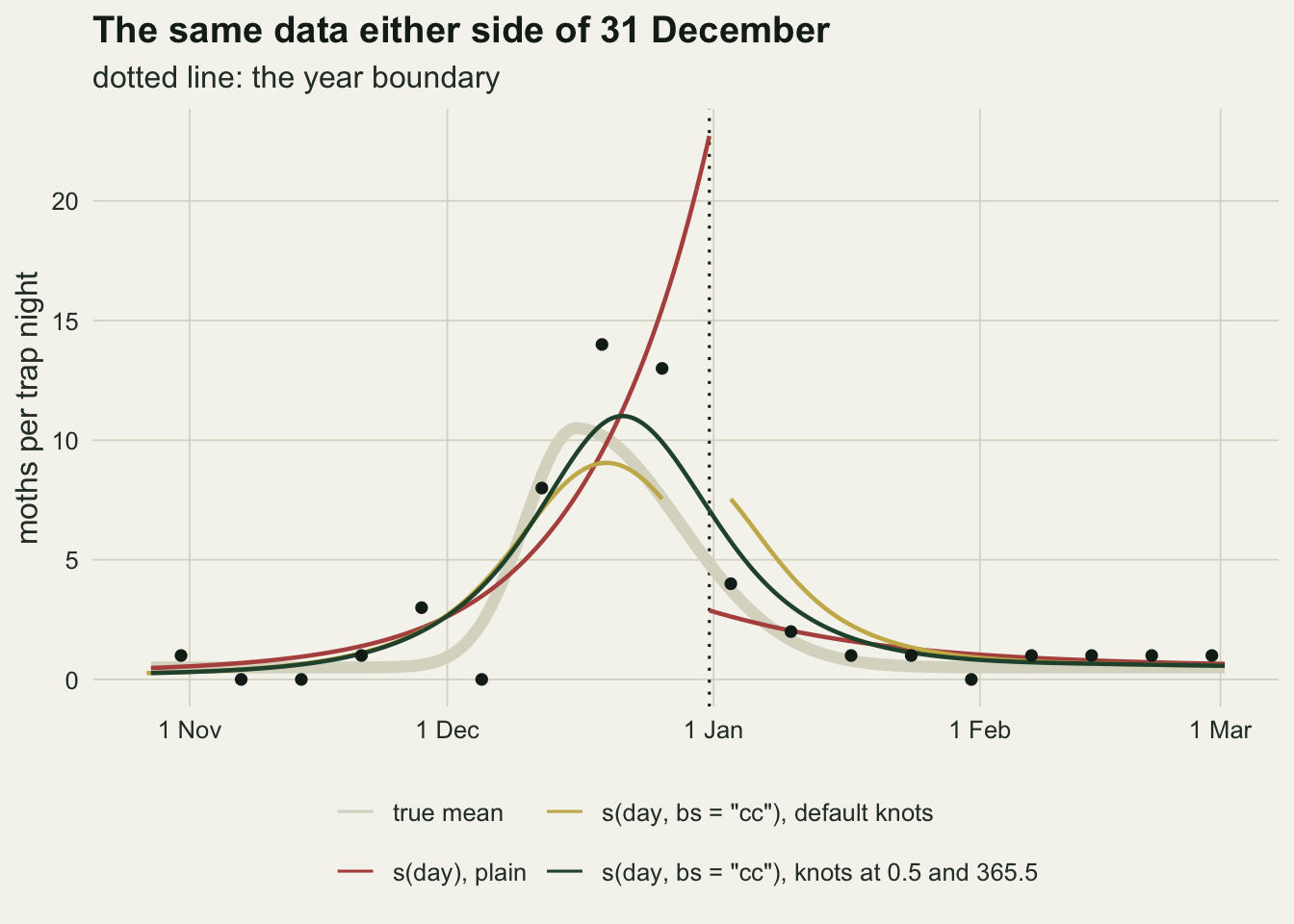

Figure 4: The same simulated season as the first figure, from 1 November to 1 March, with the year boundary marked. The plain thin plate spline fitted to day of year jumps at New Year; the cyclic spline with default end knots is drawn only between the first and last trap nights, days 3 and 360, which it joins to each other; the cyclic spline with end knots at 0.5 and 365.5 runs continuously through the boundary.

Away from the boundary the plain spline follows the year-knot cyclic spline closely, as the November and February stretches of the figure show. The damage sits at the ends, which is why it goes unnoticed when a season peaks in June; for a December pulse, or a species active through the winter, the ends are where the season is.

What to report

Say how the end knots of the cyclic smooth were set, in words and in the code. s(day, bs = "cc") without a knots argument closes the curve between the first and last observed days, not between the ends of the year, and nothing in the model summary shows which was done. With day of year coded from 1, the ends are 0.5 and 365.5; with a leap year in the data, choose a convention and state it.

When a harmonic model is used for a pulse, report the rule that chose the number of harmonics, the range searched and how often the largest value was chosen. In this design BIC chose too few harmonics to resolve a pulse three weeks wide, and a reader told only “harmonic regression” cannot tell a two-term fit from an eight-term one.

Give width and peak date with the fitting method attached, and treat a peak date from any smooth of weekly counts as uncertain by several days in the direction of the longer tail. All four fits here were late on average, so agreement between them is not evidence that the date is right.

For a cyclic spline, report the smoothing criterion as well as the basis, because on a narrow pulse it decided the width. Do not claim that a REML-fitted cyclic spline is sharper than selected harmonics; on these simulations it was not. A UBRE fit was about as sharp as AIC harmonics, but plot it against the counts before trusting its peak, since its lighter smoothing sometimes let the crest run away.

Honest limits

One pulse shape was simulated: a split Gaussian, twice as long in its fall as in its rise, with a fixed background. A symmetric pulse gives the crest no long tail to lean towards, so the date offsets here should not be carried over to it; a pulse with a flat top, or two flight periods a year, would change which harmonic count is chosen. None of these shapes was run. The ordering of the methods on width is a result for this shape and this sampling, not a general ranking.

Sampling was one trap night a week at fixed days. Daily sampling would put seven times as many points on the pulse and was not run; irregular visits, missed weeks in bad weather and effort that varies between nights were not simulated, and the last of those needs an offset or an observation model that none of these fits contains.

The counts are Poisson with no overdispersion and no year-to-year variation. Real trap counts are overdispersed, and a Poisson likelihood then overstates the information in each night, which would push AIC towards more harmonics and REML towards less smoothing; a negative binomial family for both would be the fair comparison, and it was not run. A single season is also the easy case: with several years the peak date varies between years, and a model with a cyclic smooth per year or a factor smooth, as in Hierarchical GAMs and factor smooths in mgcv, is the real tool.

The cyclic spline was fitted with REML and with UBRE, both with a single second-derivative penalty for the whole year. An adaptive smooth, which lets the penalty vary along the year, is the obvious candidate for a narrow crest on a flat background, and it might keep UBRE’s width without its runaway spikes; it was not tried in the replicate study. Nothing here says the spline family loses to harmonics: what lost was REML’s smoothing choice on this shape.

The harmonic search stopped at 8. AIC reached that limit in a minority of seasons, so a wider search would change a minority of the AIC fits; what it would do to their widths and dates was not measured.

References

Schwarz G 1978 Annals of Statistics 6(2):461-464 (10.1214/aos/1176344136)

Stolwijk AM, Straatman H, Zielhuis GA 1999 Journal of Epidemiology and Community Health 53(4):235-238 (10.1136/jech.53.4.235)

Wood SN 2011 Journal of the Royal Statistical Society Series B 73(1):3-36 (10.1111/j.1467-9868.2010.00749.x)

Wood SN 2017 Generalized Additive Models: An Introduction with R, 2nd edition (ISBN 978-1-4987-2833-1)

Related tutorials

• Harmonic regression on a seasonal raster
• Phenology in R: day of year and event timing
• Circular data and the von Mises distribution
• Choosing the basis dimension k in mgcv