library(mgcv)
library(ggplot2)

te_paper  <- "#f5f4ee"
te_ink    <- "#16241d"
te_body   <- "#2c3a31"
te_forest <- "#275139"
te_rust   <- "#b5534e"
te_gold   <- "#c9b458"
te_line   <- "#dad9ca"

theme_datasheet <- function() {
  theme_minimal(base_size = 12) +
    theme(plot.background  = element_rect(fill = te_paper, colour = NA),
          panel.background = element_rect(fill = te_paper, colour = NA),
          panel.grid.major = element_line(colour = te_line, linewidth = 0.3),
          panel.grid.minor = element_blank(),
          text             = element_text(colour = te_body),
          plot.title       = element_text(colour = te_ink, face = "bold"),
          plot.subtitle    = element_text(colour = te_body),
          axis.text        = element_text(colour = te_body),
          strip.text       = element_text(colour = te_ink, face = "bold"))
}Hierarchical GAMs and factor smooths in mgcv
R
GAMs
mgcv
smoothing
hierarchical models
thermal ecology
ecology tutorial
A by smooth fits each population alone; a factor smooth shrinks it toward a shared curve. Measuring in R what that choice does to a sparsely sampled population.
Six lake populations of a freshwater amphipod are reared across a range of temperatures, and growth rate is measured on each animal. Five lakes are easy to reach and contribute twelve animals each. The sixth is a remote upland tarn, and only eight animals from it survived the journey. The question is the same for all six: where does growth peak, and does the peak differ between lakes?
The single population version of this problem has been covered here twice. Thermal performance curves in R fits one asymmetric curve with nls and reads off the optimum. Modelling nonlinear species responses with GAMs replaces the parametric curve with a penalised smooth, and when it meets four species it loops over them with lapply, fitting four separate models that share nothing but the code. That is the right choice for four species with unrelated shapes. Six populations of one species are different. They are expected to share a curve and differ around it, and a sparsely sampled lake ought to be able to borrow the shape from the other five.
A generalised additive model can express that sharing in several ways, and mgcv offers two constructions that look almost interchangeable in a formula. s(temp, by = pop) builds one smooth per population, each with its own smoothing parameter. s(temp, pop, bs = "fs") also builds one smooth per population, but all of them share the same smoothing parameters, and the penalties cover each curve’s constant and straight line parts as well as its wiggliness, so every curve is pulled toward zero by common amounts. Pedersen, Miller, Simpson and Ross (2019) organised the combinations into five named models, and this post fits all five to simulated lakes, measures how well each recovers the true curves over repeated datasets, and checks what happens to the eight animal lake. The penalty idea underneath is the one built by hand (with a B-spline basis and GCV) in penalised regression splines from scratch. The basis size is fixed at a modest k = 6 throughout to keep the replication quick, which is smaller than the generous choice recommended in choosing the basis dimension k; the optimum section measures what that costs.
Six lakes, one of them with eight animals
Every lake follows the same asymmetric curve: a slow rise from cold water and a fall above the optimum that is twice as steep. Each lake gets its own optimum, drawn around 21 degrees, and its own vertical offset, and each animal adds measurement noise. The temperatures are drawn at random over the rearing range, separately for every animal. All of these constants were set before anything was fitted and none of them was changed afterwards.
n_grp    <- 6                       # lake populations
n_full   <- 12                      # animals in each of the first five lakes
n_sparse <- 8                       # animals from the remote tarn
k_basis  <- 6                       # basis dimension for every smooth
t_lo <- 6; t_hi <- 30               # rearing range, degrees C
opt_mu <- 21; opt_sd <- 1.5         # lake optima
lev_sd <- 0.15                      # lake offsets
sd_eps <- 0.15                      # measurement noise
w_cool <- 6; w_warm <- 3            # curve width below and above the optimum
pop_lev    <- LETTERS[seq_len(n_grp)]
sparse_pop <- pop_lev[n_grp]

tpc_true <- function(temp, opt, lev) {
  lev + exp(-0.5 * ((temp - opt) / ifelse(temp < opt, w_cool, w_warm))^2)
}

sim_pops <- function() {
  n_vec  <- c(rep(n_full, n_grp - 1), n_sparse)
  opt    <- rnorm(n_grp, opt_mu, opt_sd)
  lev    <- rnorm(n_grp, 0, lev_sd)
  pop    <- factor(rep(pop_lev, n_vec), levels = pop_lev)
  temp   <- runif(sum(n_vec), t_lo, t_hi)
  gi     <- as.integer(pop)
  growth <- tpc_true(temp, opt[gi], lev[gi]) + rnorm(length(temp), 0, sd_eps)
  list(dat = data.frame(pop, temp, growth), opt = opt, lev = lev)
}
Five ways to write the hierarchy
Pedersen et al (2019) name the models by what they contain. G is a single global smooth, with a random intercept per group. GS adds group level smooths that all share one wiggliness. GI adds group level smooths that each have their own wiggliness. S and I are the same two group level structures with the global smooth removed. The formulas below follow the ones given in the paper for its CO2 example, with the variable names changed: m = 1 on the group level by smooths of GI, which penalises the first derivative so that a linear trend in a deviation is penalised and the deviations are less collinear with the global smooth, and an explicit random intercept s(pop, bs = "re") wherever the group smooths are by smooths. A sixth formula, no_int, is model I with that intercept left out; it is not one of Pedersen’s models, and the reason for including it comes in the next section. Three more variants are fitted on part of the replication to take the models apart: GI_m2 is GI with m = 2 on its by smooths, I_id is model I with one smoothing parameter shared by all the by smooths (id = 1), and GS_k12 is GS with k = 12.
form_list <- list(
  G      = growth ~ s(temp, k = k_basis, m = 2) + s(pop, bs = "re"),
  GS     = growth ~ s(temp, k = k_basis, m = 2) +
                    s(temp, pop, bs = "fs", k = k_basis, m = 2),
  GI     = growth ~ s(temp, k = k_basis, m = 2) +
                    s(temp, by = pop, k = k_basis, m = 1) + s(pop, bs = "re"),
  S      = growth ~ s(temp, pop, bs = "fs", k = k_basis, m = 2),
  I      = growth ~ s(temp, by = pop, k = k_basis, m = 2) + s(pop, bs = "re"),
  no_int = growth ~ s(temp, by = pop, k = k_basis, m = 2)
)

# gam.side() checks nested smooths of the same variable for confounding and
# says so; for these formulas that message is expected, so only it is muted
quiet_gam <- function(form, dat) {
  withCallingHandlers(gam(form, data = dat, method = "REML"),
    warning = function(w) {
      if (grepl("repeated 1-d smooths", conditionMessage(w))) invokeRestart("muffleWarning")
    })
}
fit_forms <- function(dat) lapply(form_list, quiet_gam, dat = dat)

# variants used only to take GS, GI and I apart, fitted on part of the replication
form_extra <- list(
  GI_m2  = growth ~ s(temp, k = k_basis, m = 2) +
                    s(temp, by = pop, k = k_basis, m = 2) + s(pop, bs = "re"),
  I_id   = growth ~ s(temp, by = pop, k = k_basis, m = 2, id = 1) + s(pop, bs = "re"),
  GS_k12 = growth ~ s(temp, k = 12, m = 2) + s(temp, pop, bs = "fs", k = 12, m = 2)
)

grid_t  <- seq(t_lo, t_hi, by = 0.25)
new_pop <- expand.grid(temp = grid_t, pop = factor(pop_lev, levels = pop_lev))
opt_hat <- function(pred) {
  tapply(seq_along(pred), new_pop$pop, function(i) grid_t[which.max(pred[i])])
}
Every model is fitted by restricted maximum likelihood, the smoothing parameter estimation of Wood (2011), which treats each penalty as a variance component; Wood (2017) sets out the smooth constructions used here, including the factor by variables and the random effect basis behind s(pop, bs = "re"). One dataset first, to see what the models do before measuring how well they do it.
set.seed(620)
wk   <- sim_pops()
wdat <- wk$dat
wfit <- fit_forms(wdat)

n_sp   <- sapply(wfit, function(m) length(m$sp))
sp_I   <- wfit$I$sp[grep("s\\(temp\\)", names(wfit$I$sp))]
sp_GI  <- wfit$GI$sp[grep("s\\(temp\\):pop", names(wfit$GI$sp))]

# effective degrees of freedom of the population level smooth, lake by lake
edf_pop <- function(m, dat) {
  X   <- predict(m, type = "lpmatrix")
  out <- setNames(numeric(n_grp), pop_lev)
  for (s in m$smooth) {
    if (s$term[1] != "temp" || (length(s$term) == 1 && is.null(s$by.level))) next
    for (j in s$first.para:s$last.para) {
      lake <- unique(as.character(dat$pop[X[, j] != 0]))
      if (length(lake) == 1) out[lake] <- out[lake] + m$edf[j]
    }
  }
  out
}
edf_tab <- sapply(wfit[c("GS", "GI", "S", "I")], edf_pop, dat = wdat)

sp_GI_lake <- setNames(sp_GI, sub("s\\(temp\\):pop", "", names(sp_GI)))
n_gi_flat  <- sum(sp_GI_lake > 1e3)
tarn_min_t <- min(wdat$temp[wdat$pop == sparse_pop])
tarn_I     <- predict(wfit$I, new_pop)[new_pop$pop == sparse_pop]
tarn_I_int <- max(tarn_I[grid_t > tarn_min_t + 2])

aic_w  <- sapply(wfit, AIC)
d_aic  <- aic_w - aic_w["GS"]
wopt   <- sapply(wfit, function(m) opt_hat(predict(m, new_pop)))
tr_opt <- setNames(wk$opt, pop_lev)
The two constructions really do carry different numbers of smoothing parameters. Model I estimates 7: one for each of the 6 population smooths and one for the random intercept. Its population smooths landed on smoothing parameters ranging from 0.0015 to 0.0143, a factor of 10, and the smallest penalty of all went to lake F, the tarn. Model GS estimates 4, and only one belongs to the global smooth. The other 3 belong to the factor smooth and are shared by all six lakes: one for wiggliness and one for each of the two functions the wiggliness penalty cannot see, the constant and the straight line. The mgcv help page for the fs class states this directly: the terms are fully penalised, with a separate penalty on each null space component, and for that reason they are not centred. That is why GS needs no separate intercept term; a lake’s vertical offset is a penalised part of its deviation smooth.
The effective degrees of freedom of each lake’s own smooth show the pooling. Under model I the tarn’s smooth used 3.48 degrees of freedom, inside the range of the well sampled lakes (2.96 to 3.84), because nothing tells it to be more cautious with eight animals. Under GS its deviation from the global curve used 1.19, the lowest of the six (the others ranged from 1.62 to 1.93), and the global smooth carried the shape. Model GI pooled harder still for some lakes. In 2 of them the deviation smoothing parameter went above a thousand, the deviation smooth kept 0.00 effective degrees of freedom, and the lake was given the global curve plus an offset.
curve_df <- function(m, label) data.frame(new_pop, growth = predict(m, new_pop), model = label)
worked_curves <- rbind(curve_df(wfit$GS, "GS: shared wiggliness"),
                       curve_df(wfit$I,  "I: each lake alone"))
truth_df <- data.frame(new_pop,
  growth = tpc_true(new_pop$temp, wk$opt[as.integer(new_pop$pop)], wk$lev[as.integer(new_pop$pop)]))
lake_lab <- function(p) ifelse(p == sparse_pop, paste("Lake", p, "(8 animals)"), paste("Lake", p))

ggplot(wdat, aes(temp, growth)) +
  geom_point(colour = te_body, alpha = 0.55, size = 1.6) +
  geom_line(data = truth_df, colour = te_ink, linetype = "dashed", linewidth = 0.5) +
  geom_line(data = worked_curves, aes(colour = model), linewidth = 0.9) +
  facet_wrap(~ pop, labeller = labeller(pop = lake_lab)) +
  scale_colour_manual(values = c(te_forest, te_rust), name = NULL) +
  labs(x = "Rearing temperature (degrees C)", y = "Growth rate (relative)") +
  theme_datasheet() + theme(legend.position = "top")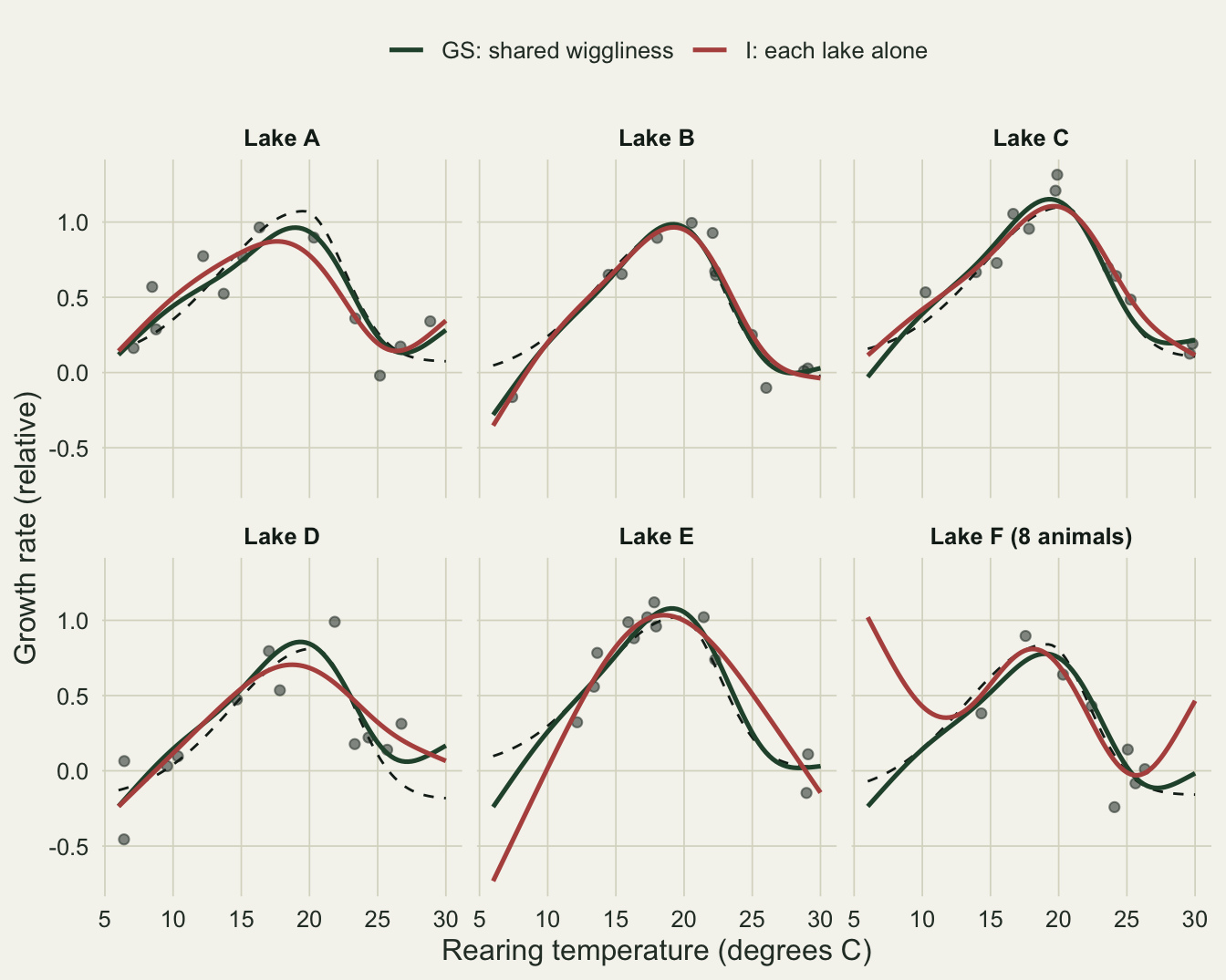
In this draw the tarn’s true optimum sits at 19.18 degrees. Model GS placed it at 19.00. Model I placed the highest point of the tarn’s curve at 6.00 degrees, the cold edge of the range. Its curve does have a hump in the right place, reaching 0.81, but the tarn’s coldest animal was reared at 14.3 degrees, and below that the smooth turned upward to 1.02 with nothing to stop it. The information criterion agrees with the picture here: model I sits 11.6 AIC units above GS. GI was lower than GS by 3.4 units and was the lowest of the five named models. One dataset is one draw, though, and the replication below is what the comparison rests on.
A by smooth has no intercept of its own
The mgcv documentation for gam.models says that when a factor is used as a by variable, centring constraints are applied to the smooths, which usually means the factor should be included as a parametric term as well. The exact form of the constraint is worth knowing. In mgcv 1.9 the sum to zero constraint for a smooth is computed from the basis evaluated at every row of the data, and only then is the smooth copied once per level and multiplied by the level indicator. So each population’s curve is constrained to average zero over the temperatures of all animals in the dataset, not over its own animals. Leave out the intercept term and every population’s fitted curve, averaged over the pooled temperatures, equals the model intercept.
no_int <- wfit$no_int
pooled <- data.frame(temp = rep(wdat$temp, n_grp),
                     pop  = factor(rep(pop_lev, each = nrow(wdat)), levels = pop_lev))
pooled_mean <- tapply(predict(no_int, pooled), pooled$pop, mean)
icpt        <- unname(coef(no_int)[1])
max_gap     <- max(abs(pooled_mean - icpt))

own_mean <- tapply(fitted(no_int), wdat$pop, mean)
obs_mean <- tapply(wdat$growth, wdat$pop, mean)

# the form in the mgcv help: a fixed factor term instead of a random intercept
m_fixed   <- quiet_gam(growth ~ pop + s(temp, by = pop, k = k_basis), wdat)
fixed_gap <- max(abs(tapply(fitted(m_fixed), wdat$pop, mean) - obs_mean))

rmse_grid <- function(m) {
  sqrt(tapply((predict(m, new_pop) - truth_df$growth)^2, new_pop$pop, mean))
}
rm_noint <- rmse_grid(no_int)
rm_I     <- rmse_grid(wfit$I)
The intercept of the model without a population term is 0.5125, and the six population curves averaged over the pooled temperatures differ from it by at most 4.27e-13, which is rounding error. Averaged over each lake’s own animals the fitted values are not forced to be equal, because each lake’s temperatures are a different random sample: they range from 0.291 to 0.683, against observed lake means from 0.272 to 0.717. The loss is the vertical offset. A lake that grows faster at every temperature cannot be represented by a curve that must average to the common intercept over the same temperatures as everyone else, so the smooth bends to fake the offset. With the fixed factor term of the help page restored, the least squares equations for the unpenalised factor columns force each lake’s mean fitted value to equal its observed mean, and the largest discrepancy is 4.44e-16.
cent_curves <- rbind(curve_df(wfit$I,  "I: by smooths plus intercept"),
                     curve_df(no_int, "no_int: by smooths only"))
ggplot(wdat, aes(temp, growth)) +
  geom_point(colour = te_body, alpha = 0.55, size = 1.6) +
  geom_line(data = truth_df, colour = te_ink, linetype = "dashed", linewidth = 0.5) +
  geom_hline(yintercept = icpt, colour = te_gold, linewidth = 0.6) +
  geom_line(data = cent_curves, aes(colour = model), linewidth = 0.9) +
  facet_wrap(~ pop, labeller = labeller(pop = lake_lab)) +
  scale_colour_manual(values = c(te_forest, te_rust), name = NULL) +
  labs(x = "Rearing temperature (degrees C)", y = "Growth rate (relative)") +
  theme_datasheet() + theme(legend.position = "top")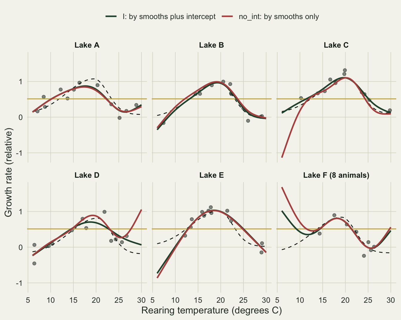
In this dataset the damage is largest for lake C, where the error against the true curve rose from 0.065 to 0.318, and for lake D the curve without an intercept put its highest point at 30.00 degrees, the warm edge, against a true optimum of 20.31. The model fits without complaint and prints no warning about it.
Repeated datasets: who recovers the curves
The worked dataset shows mechanisms. The ranking needs many datasets. Each replicate draws six new lakes, fits all six formulas, and records the root mean squared difference between each fitted curve and the lake’s true curve over the rearing range, the temperature of the fitted peak, and the AIC.
n_rep <- 150
n_sub <- 75     # the first n_sub datasets also get the three variants and ML refits
set.seed(4077)
rep_rows <- lapply(seq_len(n_rep), function(r) {
  sim   <- sim_pops()
  fits  <- fit_forms(sim$dat)
  aic_ml <- setNames(rep(NA_real_, length(form_list)), names(form_list))
  if (r <= n_sub) {
    fits <- c(fits, lapply(form_extra, quiet_gam, dat = sim$dat))
    for (nm in c("GS", "I")) {
      aic_ml[nm] <- AIC(withCallingHandlers(gam(form_list[[nm]], data = sim$dat, method = "ML"),
        warning = function(w) {
          if (grepl("repeated 1-d smooths", conditionMessage(w))) invokeRestart("muffleWarning")
        }))
    }
  }
  gi    <- as.integer(new_pop$pop)
  truth <- tpc_true(new_pop$temp, sim$opt[gi], sim$lev[gi])
  do.call(rbind, lapply(names(fits), function(nm) {
    pred <- predict(fits[[nm]], new_pop)
    data.frame(rep = r, model = nm, pop = pop_lev,
               rmse    = sqrt(as.vector(tapply((pred - truth)^2, new_pop$pop, mean))),
               opt_err = as.vector(opt_hat(pred)) - sim$opt,
               opt_edge = as.vector(opt_hat(pred)) %in% c(t_lo, t_hi),
               aic     = AIC(fits[[nm]]),
               aic_ml  = if (nm %in% names(aic_ml)) aic_ml[[nm]] else NA_real_)
  }))
})
rep_all <- do.call(rbind, rep_rows)
rep_sub <- rep_all[rep_all$rep <= n_sub, ]
rep_all <- rep_all[rep_all$model %in% names(form_list), ]
rep_all$group <- ifelse(rep_all$pop == sparse_pop, "Tarn (8 animals)", "Other five lakes (12 each)")

by_rep <- aggregate(rmse ~ model + rep + group, data = rep_all, FUN = mean)
rmse_sum <- do.call(rbind, lapply(split(by_rep, list(by_rep$model, by_rep$group)), function(d) {
  data.frame(model = d$model[1], group = d$group[1],
             mean = mean(d$rmse), se = sd(d$rmse) / sqrt(nrow(d)))
}))
wide <- reshape(by_rep, idvar = c("rep", "group"), timevar = "model", direction = "wide")
pair_diff <- function(a, b, grp, wd = wide) {
  w  <- wd[wd$group == grp, ]
  dd <- w[[paste0("rmse.", a)]] - w[[paste0("rmse.", b)]]
  c(diff = mean(dd), se = sd(dd) / sqrt(length(dd)), share = mean(dd > 0),
    rel = mean(dd) / mean(w[[paste0("rmse.", a)]]))
}
g_full <- "Other five lakes (12 each)"; g_tarn <- "Tarn (8 animals)"
IvGS_f  <- pair_diff("I", "GS", g_full);  IvGS_t  <- pair_diff("I", "GS", g_tarn)
IvS_f   <- pair_diff("I", "S", g_full);   IvS_t   <- pair_diff("I", "S", g_tarn)
SvGS_f  <- pair_diff("S", "GS", g_full);  SvGS_t  <- pair_diff("S", "GS", g_tarn)
GIvGS_f <- pair_diff("GI", "GS", g_full); GIvGS_t <- pair_diff("GI", "GS", g_tarn)
NIvI_f  <- pair_diff("no_int", "I", g_full)
rm_mean <- function(mod, grp) rmse_sum$mean[rmse_sum$model == mod & rmse_sum$group == grp]

# the first n_sub datasets, where the variants were also fitted
rep_sub$group <- ifelse(rep_sub$pop == sparse_pop, g_tarn, g_full)
wide_sub <- reshape(aggregate(rmse ~ model + rep + group, data = rep_sub, FUN = mean),
                    idvar = c("rep", "group"), timevar = "model", direction = "wide")
sub_mean <- function(mod, grp) mean(wide_sub[wide_sub$group == grp, paste0("rmse.", mod)])
GIm2vGI_f <- pair_diff("GI_m2", "GI", g_full, wide_sub); GIm2vGI_t <- pair_diff("GI_m2", "GI", g_tarn, wide_sub)
GIm2vGS_f <- pair_diff("GI_m2", "GS", g_full, wide_sub); GIm2vGS_t <- pair_diff("GI_m2", "GS", g_tarn, wide_sub)
IvIid_f   <- pair_diff("I", "I_id", g_full, wide_sub);   IvIid_t   <- pair_diff("I", "I_id", g_tarn, wide_sub)
IidvS_f   <- pair_diff("I_id", "S", g_full, wide_sub);   IidvS_t   <- pair_diff("I_id", "S", g_tarn, wide_sub)
id_share_f <- IvIid_f["diff"] / (IvIid_f["diff"] + IidvS_f["diff"])rmse_sum$model <- factor(rmse_sum$model, levels = rev(c("G", "GS", "GI", "S", "I", "no_int")))
ggplot(rmse_sum, aes(mean, model)) +
geom_errorbar(aes(xmin = mean - 2 * se, xmax = mean + 2 * se), orientation = "y",
width = 0.25, colour = te_body, linewidth = 0.5) +
geom_point(aes(colour = model %in% c("GS", "GI")), size = 2.8) +
facet_wrap(~ group) +
scale_colour_manual(values = c(`TRUE` = te_forest, `FALSE` = te_rust), guide = "none") +
labs(x = "Root mean squared error against the true curve", y = NULL) +
theme_datasheet()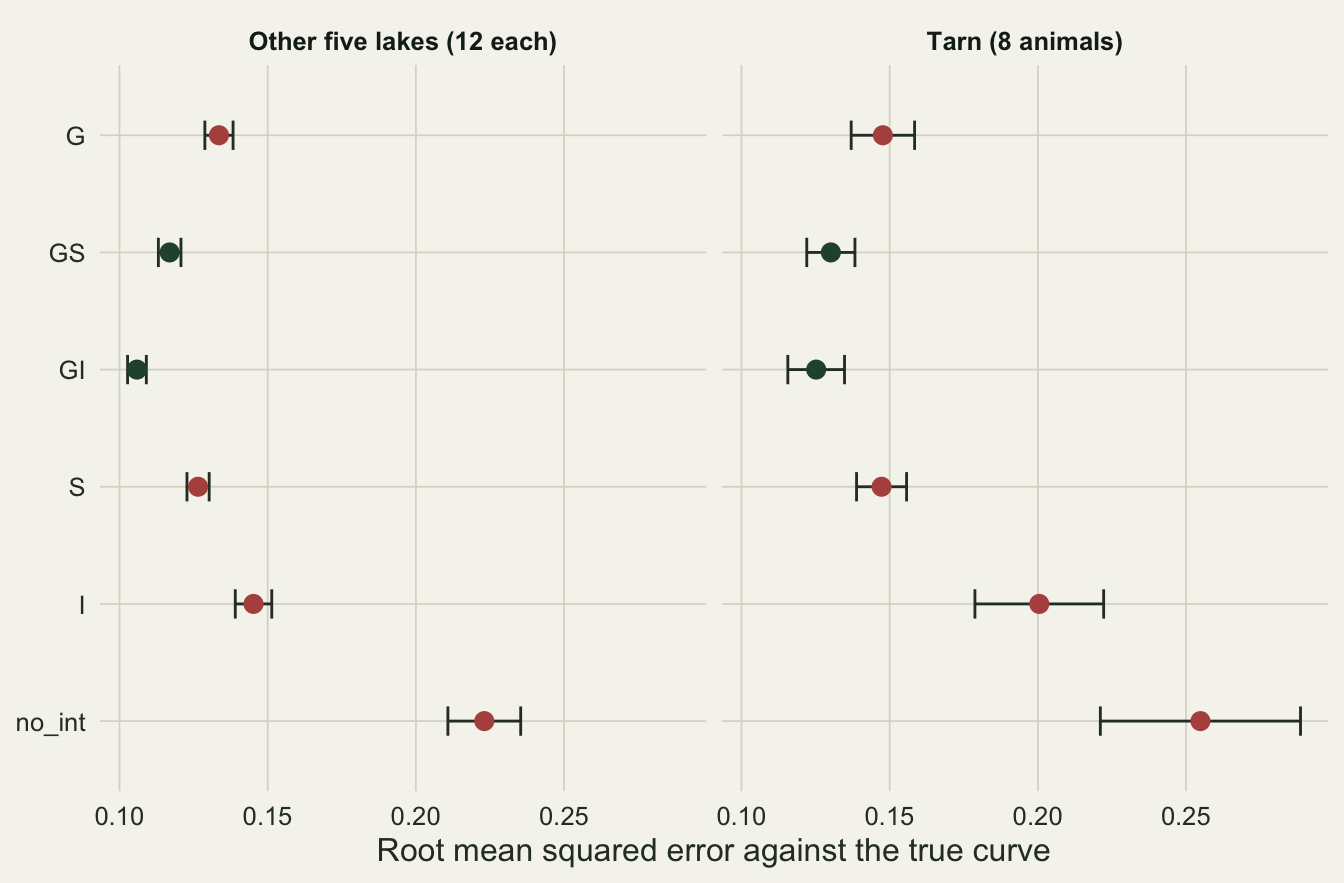
Across 150 datasets, model I’s error for the well sampled lakes averaged 0.1452 against 0.1169 for GS, so sharing the wiggliness and adding the global curve cut the error by 19 per cent (paired difference 0.0283, standard error 0.0031). For the tarn the same comparison was 0.2005 against 0.1302, a cut of 35 per cent (difference 0.0703, standard error 0.0109). The gain is larger for the sparsely sampled lake, as expected, but it is not confined to it: GS beat I for the well sampled lakes in 83 per cent of datasets.
The two ingredients of GS can be separated. Model S shares the wiggliness but has no global smooth. Against I it lowered the error by 13 per cent for the five lakes and 27 per cent for the tarn; adding the global smooth, S to GS, lowered it by a further 8 and 12 per cent. Both parts help. But S differs from I in a second way as well: the factor smooth also penalises each lake’s constant and straight line, while I’s by smooths keep an unpenalised straight line per lake next to a separate random intercept. The variant I_id, fitted on the first 75 datasets, shares one smoothing parameter across I’s by smooths but keeps those unpenalised lines, so it sits between the two. Sharing the smoothing parameter, I to I_id, lowered the error by 0.0139 (standard error 0.0024) for the five lakes and 0.0190 (0.0060) for the tarn. Penalising the constant and the line as well, I_id to S, lowered it by a further 0.0063 (0.0026) and 0.0159 (0.0067). For the five lakes the shared smoothing parameter accounts for 69 per cent of the I to S gain and the null space penalty for the rest; for the tarn the second step is not separated from zero.
The one result that goes against the story as usually told is GI. It gives every lake its own smoothing parameter, which is exactly what hurt model I, yet it had the lowest error of all six formulas for the well sampled lakes, below GS by 0.0110 (standard error 0.0013). For the tarn it was also lower on average, by 0.0050, but with a standard error of 0.0044 that difference is not separated from zero. So separate smoothing parameters hurt model I, as the I_id step showed, but did not hurt GI, and the global smooth does not explain that difference on its own either. The variant GI_m2, which is GI with m = 2 on its by smooths, had a mean error of 0.1286 for the five lakes over the first 75 datasets, against 0.1064 for GI and 0.1158 for GS: above GI by 0.0222 (standard error 0.0025) and above GS by 0.0128 (0.0029). For the tarn it was above GI by 0.0202 (0.0052), and its difference from GS, 0.0088 (0.0067), is not separated from zero. What GI adds is m = 1. With m = 1 the only function the penalty cannot see is the constant, and the centring constraint removes the constant from each by smooth, so the deviation that remains is fully penalised: a large smoothing parameter shrinks it to zero and leaves the lake with the global curve plus its random intercept, as happened to 2 lakes in the worked dataset. A by smooth with m = 2 always keeps an unpenalised straight line per lake. Leaving out the intercept term cost more than any modelling choice among Pedersen’s five: for the five lakes no_int averaged 0.2231 against 0.1452 for model I.
The tarn’s optimum
The applied question was where growth peaks. For the tarn, the error of the estimated optimum is summarised below as the mean absolute error, the mean signed error, and the share of datasets in which the estimate was more than four degrees from the truth.
tarn  <- rep_all[rep_all$pop == sparse_pop, ]
opt_tab <- do.call(rbind, lapply(split(tarn, tarn$model), function(d) {
  data.frame(model = d$model[1], mae = mean(abs(d$opt_err)), bias = mean(d$opt_err),
             wild = mean(abs(d$opt_err) > 4),
             edge_of_wild = mean(d$opt_edge[abs(d$opt_err) > 4]))
}))
rownames(opt_tab) <- opt_tab$model
wild_se <- function(p) sqrt(p * (1 - p) / n_rep)
five  <- rep_all[rep_all$pop != sparse_pop, ]
bias_five <- tapply(five$opt_err, five$model, mean)

# basis or penalty: GS with k = 6 and k = 12 on the same n_sub datasets, all six lakes
bias_rep <- aggregate(opt_err ~ rep + model, data = rep_sub[rep_sub$model %in% c("GS", "GS_k12"), ],
                      FUN = mean)
bias_w   <- reshape(bias_rep, idvar = "rep", timevar = "model", direction = "wide")
bias_k6  <- mean(bias_w$opt_err.GS)
bias_k12 <- mean(bias_w$opt_err.GS_k12)
bias_k6_se  <- sd(bias_w$opt_err.GS) / sqrt(n_sub)
bias_k12_se <- sd(bias_w$opt_err.GS_k12) / sqrt(n_sub)
bias_shift    <- mean(bias_w$opt_err.GS_k12 - bias_w$opt_err.GS)
bias_shift_se <- sd(bias_w$opt_err.GS_k12 - bias_w$opt_err.GS) / sqrt(n_sub)

# no noise, no lakes: the k = 6 smooth fitted to the true curve itself
temp_fine <- seq(t_lo, t_hi, length.out = 400)
clean  <- data.frame(temp = temp_fine, growth = tpc_true(temp_fine, opt_mu, 0))
peak_k <- sapply(c(6, 12), function(kk) {
  temp_fine[which.max(fitted(gam(growth ~ s(temp, k = kk), data = clean)))]
})
sp_clean6 <- gam(growth ~ s(temp, k = 6), data = clean)$sp
peak_fx6 <- temp_fine[which.max(fitted(gam(growth ~ s(temp, k = 6, fx = TRUE), data = clean)))]tarn$model <- factor(tarn$model, levels = rev(c("G", "GS", "GI", "S", "I", "no_int")))
ggplot(tarn, aes(opt_err, model)) +
geom_vline(xintercept = 0, colour = te_ink, linetype = "dashed", linewidth = 0.4) +
geom_jitter(height = 0.18, width = 0, alpha = 0.35, size = 1.2,
colour = ifelse(tarn$model %in% c("GS", "GI"), te_forest, te_rust)) +
stat_summary(fun = median, fun.min = median, fun.max = median, geom = "crossbar",
width = 0.55, colour = te_ink, linewidth = 0.4) +
labs(x = "Estimated minus true optimum (degrees C)", y = NULL) +
theme_datasheet()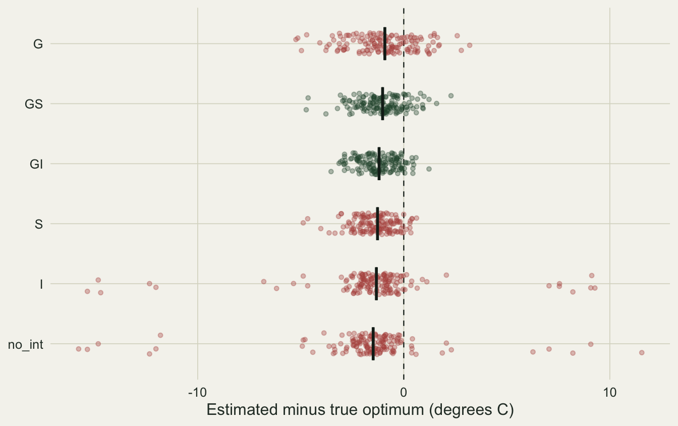
Model I missed the tarn’s optimum by 2.24 degrees on average, and its estimate was more than four degrees out in 11.3 per cent of datasets (Monte Carlo standard error 2.6 points); in 71 per cent of those wild estimates the maximum of the fitted curve sat on an edge of the rearing range, the failure seen in the worked dataset. GS missed by 1.27 degrees with 1.3 per cent wild estimates, and GI by 1.28 degrees with 0.0 per cent.
The figure also shows something no choice of hierarchy repairs. The bulk of every model’s estimates sits to the left of zero: the mean signed error was -1.08 degrees for GS, -1.22 for GI and -1.39 for I, and for the five well sampled lakes the models ranged from -1.40 to -1.12. How much of that is the basis and how much the penalty can be measured. A k = 6 smooth fitted to the noise free true curve, with an optimum at 21 degrees, peaks at 19.83. Its smoothing parameter is 7.70e-05, and the same basis with no penalty at all (fx = TRUE) peaks at 19.83, so that shortfall is basis truncation alone. With k = 12 the noise free peak is at 20.68, which predicts a shift of 0.84 degrees from the larger basis. On the first 75 datasets GS was refitted with k = 12. Its mean signed error over all six lakes moved from -1.26 (standard error 0.05) to -1.08 (0.06), a paired shift of 0.18 (standard error 0.03). With k = 6, the noise free truncation of 1.17 degrees is most of the 1.26; with k = 12 it is only 0.32 of the 1.08. The rest appears with sparse, noisy data, where REML smooths the sharp peak toward its gentle cold side. The subtraction is not a clean split between basis and penalty, though: the check used a dense, evenly spaced, noise free curve, not twelve or fewer random temperatures per lake, so part of the remainder may still be truncation. Most of the bias stayed. Hierarchical pooling reduces the scatter of the optimum; neither the choice of hierarchy nor a larger basis removed this smoothing bias.
aics <- unique(rep_all[rep_all$model != "no_int", c("rep", "model", "aic")])
aic_w5 <- reshape(aics, idvar = "rep", timevar = "model", direction = "wide")
five_names <- c("G", "GS", "GI", "S", "I")
aic_best <- five_names[apply(aic_w5[, paste0("aic.", five_names)], 1, which.min)]
tot <- aggregate(rmse ~ model + rep, data = rep_all[rep_all$model != "no_int", ], FUN = mean)
tot_w <- reshape(tot, idvar = "rep", timevar = "model", direction = "wide")
rmse_best <- five_names[apply(tot_w[, paste0("rmse.", five_names)], 1, which.min)]
aic_agree  <- mean(aic_best == rmse_best)
aic_GI     <- mean(aic_best == "GI")
aic_I_lt   <- mean(aic_w5$aic.I < aic_w5$aic.GS)
rmse_I_gt  <- mean(tot_w$rmse.I > tot_w$rmse.GS)
d_aic_I    <- mean(aic_w5$aic.I - aic_w5$aic.GS)

# the same comparison on the first n_sub datasets, REML fits against ML refits
aic_s  <- unique(rep_sub[rep_sub$model %in% c("GS", "I"), c("rep", "model", "aic", "aic_ml")])
aic_sw <- reshape(aic_s, idvar = "rep", timevar = "model", direction = "wide")
aic_I_lt_reml <- mean(aic_sw$aic.I < aic_sw$aic.GS)
aic_I_lt_ml   <- mean(aic_sw$aic_ml.I < aic_sw$aic_ml.GS)
d_aic_I_reml  <- mean(aic_sw$aic.I - aic_sw$aic.GS)
d_aic_I_ml    <- mean(aic_sw$aic_ml.I - aic_sw$aic_ml.GS)
AIC is a weak guide to this choice. The values here are mgcv’s AIC from the REML fits, which counts the effective degrees of freedom with the correction for smoothing parameter uncertainty described on the logLik.gam help page. It picked GI in 63 per cent of datasets, which is defensible, but it picked the same model as the error against the truth in only 47 per cent. It preferred model I to GS in 65 per cent of datasets, with a mean difference of -2.91 units in favour of I, although I recovered the curves less well than GS in 87 per cent. The verdict also depends on the fitting method. On the first 75 datasets the REML fits preferred I to GS in 65 per cent, with a mean difference of -3.84; with both models refitted by maximum likelihood the share was 49 per cent and the mean difference 1.36. The AIC for a penalised model counts the effective degrees of freedom the penalty left behind, and it scores how well the fit reproduces the animals that were measured; the error against the true curve is about the lakes, including the parts of the tarn’s range where there were no animals. Tensor product smooths in mgcv found the REML score a similarly poor compass for choosing between s() and te().
What to report
Report the formula, not the phrase “hierarchical GAM”, because the five models behave differently and the words do not tell a reader which one was fitted. State for each group level smooth whether its smoothing parameter is shared, and whether there is a global smooth. If group level by smooths are used, include a group intercept, either as a fixed factor term or as s(group, bs = "re"), and say which.
Report the number of observations per group next to each group’s estimate, and the effective degrees of freedom of that group’s smooth. A group estimate that carries as many degrees of freedom as the well sampled groups while resting on two thirds of their data is a warning sign in its own right. When a derived quantity such as an optimum is the result, state the basis dimension and check it with k.check and a refit with a larger basis. Do not expect the larger basis to remove the bias of a sharp peak: here it removed only a small part, and with few observations per group the smoothing that REML chooses also flattens the peak toward its gentle side. Say so next to the estimate.
Do not choose among these structures by AIC alone. Choose on what the groups are expected to share, which is a statement about biology before it is a statement about fit.
Honest limits
The truth was simulated from exactly the situation the hierarchical models are built for: six lakes sharing one curve shape, with optima and offsets drawn from a common distribution. If the lakes had genuinely different shapes, for example one with a second peak, a shared penalty would oversmooth the odd one out, and model I, which was worst here, could be the right choice. No such scenario was simulated.
The design is one point. Six groups, twelve animals in five of them and eight in the sixth, a Gaussian response, temperatures spread at random over the whole range for every lake. A tarn whose eight animals all came from the cold half of the range would test a different thing, the ability of the global curve to extrapolate a lake’s deviation, and the numbers above do not describe it. With six groups the random intercept and the shared smoothing parameters are estimated from very few levels, which is the setting of random effects with too few levels; the results were not checked with more groups.
The replication is 150 datasets, chosen to keep the whole post quick to run. The variants GI_m2, I_id and GS_k12 and the maximum likelihood refits used only the first 75 of them, so their comparisons carry larger standard errors. The full replication separates GS from I and GI from GS for the well sampled lakes, but it does not separate GI from GS for the tarn, and the rates of wild optimum estimates carry Monte Carlo standard errors of a few percentage points.
The basis dimension was fixed at 6 for every smooth, global and group level alike, below the generous choice the k tutorial recommends. Only GS was refitted with k = 12, and only to measure the optimum bias; the other models were not, so whether a larger basis would change the ranking of the models was not measured. Pedersen et al (2019) discuss letting the global and group level smooths have different basis sizes, which was not tried here either.
Finally, mgcv offers a construction not tested here: the "sz" factor smooth, which constrains the group level smooths so that their equivalent coefficients sum to zero across groups. The mgcv help contrasts the two directly: with "fs" a model with a main effect plus group deviations can be built, but the model is not forced to make the main effect do as much of the work as possible, and with "sz" it is. That is the natural next comparison.
References
Pedersen EJ, Miller DL, Simpson GL, Ross N 2019 PeerJ 7:e6876 (10.7717/peerj.6876)
Wood SN 2011 Journal of the Royal Statistical Society Series B 73(1):3-36 (10.1111/j.1467-9868.2010.00749.x)
Wood SN 2017 Generalized Additive Models: An Introduction with R, 2nd edition (ISBN 978-1-4987-2833-1)