library(ggplot2)
library(patchwork)
library(mgcv)

te_paper  <- "#f5f4ee"
te_ink    <- "#16241d"
te_body   <- "#2c3a31"
te_forest <- "#275139"
te_rust   <- "#b5534e"
te_gold   <- "#c9b458"
te_line   <- "#dad9ca"

theme_datasheet <- function() {
  theme_minimal(base_size = 12) +
    theme(plot.background  = element_rect(fill = te_paper, colour = NA),
          panel.background = element_rect(fill = te_paper, colour = NA),
          panel.grid.major = element_line(colour = te_line, linewidth = 0.3),
          panel.grid.minor = element_blank(),
          text             = element_text(colour = te_body),
          plot.title       = element_text(colour = te_ink, face = "bold"),
          plot.subtitle    = element_text(colour = te_body),
          axis.text        = element_text(colour = te_body))
}Tensor product smooths in mgcv
R
mgcv
GAMs
spatial ecology
ecology tutorial
An isotropic s(x, z) on covariates with different scales hides a unit choice. Measuring what te() buys in mgcv, and when isotropy is the right claim to make.
A towed camera sled runs one straight line out across the shelf, logging where it is along the transect and how deep the water is beneath it. Every still is scored for the cover of a habitat forming sponge, and the question is how that cover changes with position along the line and with depth. In mgcv the model that answers both at once is a single two-dimensional smooth, and almost everyone writes it the same way: gam(cover ~ s(dist, depth)).
The transect is kilometres long and the depth range is tens of metres. Both covariates are recorded in metres, so nothing about that call looks suspicious. But s(dist, depth) builds a thin plate regression spline (Wood 2003), and the thin plate penalty is isotropic: it charges the same price for wiggliness in any direction on the plane the two covariates span. Writing that formula asserts that one metre along the line is exchangeable with one metre of depth. That is a claim about the seabed, not about the software, and nothing in the output flags it.
This post makes the claim visible by rescaling the along-transect covariate by a factor and refitting. The factor carries no science: it converts metres into some other unit. What it does carry is out-of-sample error, and sweeping it traces a U-shaped curve with metres and kilometres both on the wrong part of it. A tensor product smooth, te(), builds the same surface from two one-dimensional bases with a separate smoothing parameter for each, and its answer does not move with the factor at all. That invariance is an algebraic identity rather than a lucky result, and the machine-precision check below is here so it can be verified rather than believed. A later section measures what te() costs when isotropy really is the right assumption, because it does cost something.
This is the companion to choosing the basis dimension k: that post asks how much wiggliness the basis is allowed, this one asks what shape the wiggliness is allowed to take. The density surface model post fits s(line, ymid, k = 20) with both coordinates in kilometres, which is the case where the isotropic choice is right, and it never says so; the spatial cross-validation post uses the same construction on synthetic grid coordinates for a different question entirely. Anisotropy in the geostatistical sense already has a home on this site under directional variograms and kriging, where correlation reaches further along a valley than across it. The point here is that the same asymmetry has to be handled in the smoothing basis, and that a variogram is not the only place it hides.
A metre along the transect is not a metre of depth
The truth is a known function, so error can be measured against the noiseless surface rather than against noisy observations. It is built from one sine wave along each axis plus a product term, and it completes more cycles along the transect than across the depth range.
span_x  <- 2000; span_z  <- 40    # metres of transect, metres of depth
wu_base <- 1.5;  wv_base <- 0.5   # cycles of the truth across each span
truth <- function(x, z, wu = wu_base, wv = wv_base) {
  u <- x / span_x; v <- z / span_z
  sin(2 * pi * wu * u + 0.4) + 0.9 * sin(2 * pi * wv * v) +
    1.1 * sin(2 * pi * wu * u) * sin(2 * pi * wv * v)
}
mc_se <- function(v) sd(v) / sqrt(length(v))
n_train <- 400; n_test <- 1000; noise_sd <- 0.5; k_marg <- 8
aniso <- wu_base / wv_base; km_factor <- 1000
400 stills over 2000 metres of transect and 40 metres of depth, with Gaussian noise of standard deviation 0.5. The truth completes 1.5 cycles along the transect against 0.5 across the depth range, so it is 3 times as wiggly per unit of span in distance as in depth. Fit quality is out-of-sample root mean squared error against the truth at 1000 fresh points, so nothing is scored on the data it was fitted to. The rescaling divides the distance covariate and leaves depth alone: a factor of one is metres, a factor of 1000 is kilometres, and the values between and beyond are units nobody would name. The two smoothers are matched on basis size, 64 functions for s() against 8 per margin for te().
cs <- c(0.01, 1, 3, 10, 17, 30, 100, 1000, 10000)
n_rep <- 12; seed_sweep <- 2250

draw_survey <- function(wu = wu_base, wv = wv_base, sd_e = noise_sd) {
  tr <- data.frame(x = runif(n_train, 0, span_x), z = runif(n_train, 0, span_z))
  tr$y <- truth(tr$x, tr$z, wu, wv) + rnorm(n_train, 0, sd_e)
  ho <- data.frame(x = runif(n_test, 0, span_x), z = runif(n_test, 0, span_z))
  ho$f <- truth(ho$x, ho$z, wu, wv); list(tr = tr, ho = ho)
}
score_fit <- function(fm, tr, ho) {
  fit <- gam(fm, data = tr, method = "REML")
  c(sqrt(mean((as.numeric(predict(fit, ho)) - ho$f)^2)),
    sum(fit$edf) - 1, unname(fit$gcv.ubre))
}
rows <- list()
for (r in seq_len(n_rep)) {
  set.seed(seed_sweep + r)
  dd <- draw_survey(); tr <- dd$tr; ho <- dd$ho
  for (cc in cs) {
    tr$xs <- tr$x / cc; ho$xs <- ho$x / cc
    v_iso <- score_fit(y ~ s(xs, z, k = k_marg^2), tr, ho)
    v_ten <- score_fit(y ~ te(xs, z, k = c(k_marg, k_marg)), tr, ho)
    rows[[length(rows) + 1]] <- data.frame(rep = r, cc = cc,
      s_rmse = v_iso[1], s_edf = v_iso[2], s_reml = v_iso[3],
      t_rmse = v_ten[1], t_edf = v_ten[2])
  }
}
sw <- do.call(rbind, rows)
agg <- do.call(rbind, lapply(cs, function(cc) {
  d <- sw[sw$cc == cc, ]
  data.frame(cc = cc, s_rmse = mean(d$s_rmse), s_se = mc_se(d$s_rmse),
             s_edf = mean(d$s_edf), t_rmse = mean(d$t_rmse), t_se = mc_se(d$t_rmse),
             t_edf = mean(d$t_edf), paired = mean(d$s_rmse - d$t_rmse),
             paired_se = mc_se(d$s_rmse - d$t_rmse), ratio = mean(d$s_rmse) / mean(d$t_rmse))
}))
i_m <- which(cs == 1); i_km <- which(cs == 1000); j_best <- which.min(agg$s_rmse)
rmse_metres <- agg$s_rmse[i_m]; rmse_km <- agg$s_rmse[i_km]
ratio_metres <- agg$ratio[i_m]; ratio_km <- agg$ratio[i_km]; edf_lo <- min(agg$s_edf)
ten_rmse <- mean(agg$t_rmse); ten_se <- mean(agg$t_se); ten_edf <- mean(agg$t_edf)
c_best <- agg$cc[j_best]; rmse_bst <- agg$s_rmse[j_best]; se_bst <- agg$s_se[j_best]
c_worst <- agg$cc[which.max(agg$s_rmse)]; rmse_wst <- max(agg$s_rmse)
span_ratio <- rmse_wst / rmse_bst; c_edf_hi <- agg$cc[which.max(agg$s_edf)]
edf_hi <- max(agg$s_edf); c_star_pred <- span_x * wv_base / (span_z * wu_base)
opt_paired <- agg$paired[j_best]; opt_paired_se <- agg$paired_se[j_best]
opt_sigma <- opt_paired / opt_paired_se
At metres the isotropic fit scores 0.4381 and at kilometres 1.1136, against 0.1354 for the tensor product. Metres is the better of the two unit choices here by a factor of 2.54, but that ordering is a property of this particular seabed and not a rule: it says only that stretching the transect axis hurts less than compressing it when the truth is wigglier along the transect than down the depth range.
The unit choice is a curve, not a mistake
Neither metres nor kilometres is a candidate for the right answer, so reporting the ratio between them would be reporting one arbitrary comparison; the full sweep is the honest object. Over the swept range the isotropic fit runs from 0.1410 at a factor of 17 to 1.1497 at a factor of 10000, a spread of 8.15 times in root mean squared error. Every point on that curve is the same data, the same basis size and the same estimation method. The only thing that changed was a unit.
panel_c <- function(yv, flat, ylab, ttl, sub_ttl, se_y = NULL) {
  p <- ggplot(data.frame(cc = agg$cc, y = yv), aes(cc, y))
  if (!is.null(se_y)) p <- p +
    geom_vline(xintercept = c(1, km_factor), colour = te_body,
               linetype = "dotted", linewidth = 0.4) +
    geom_ribbon(aes(ymin = y - se_y, ymax = y + se_y), fill = te_rust, alpha = 0.18)
  p + geom_line(colour = te_rust, linewidth = 0.9) +
    geom_point(colour = te_rust, size = 2) +
    geom_hline(yintercept = flat, colour = te_forest,
               linetype = "dashed", linewidth = 0.8) +
    scale_x_log10(breaks = c(0.01, 1, 100, 10000), labels = function(v)
                    format(v, scientific = FALSE, trim = TRUE, drop0trailing = TRUE)) +
    labs(x = "rescaling factor on distance", y = ylab, title = ttl, subtitle = sub_ttl) +
    theme_datasheet()
}

panel_c(agg$s_rmse, ten_rmse, "out of sample RMSE", "Error",
        "red: s(); green dashed: te()", se_y = agg$s_se) +
  panel_c(agg$s_edf, ten_edf, "effective degrees of freedom", "Flexibility used",
          "the same fits, counted differently") +
  plot_annotation(theme = theme_datasheet())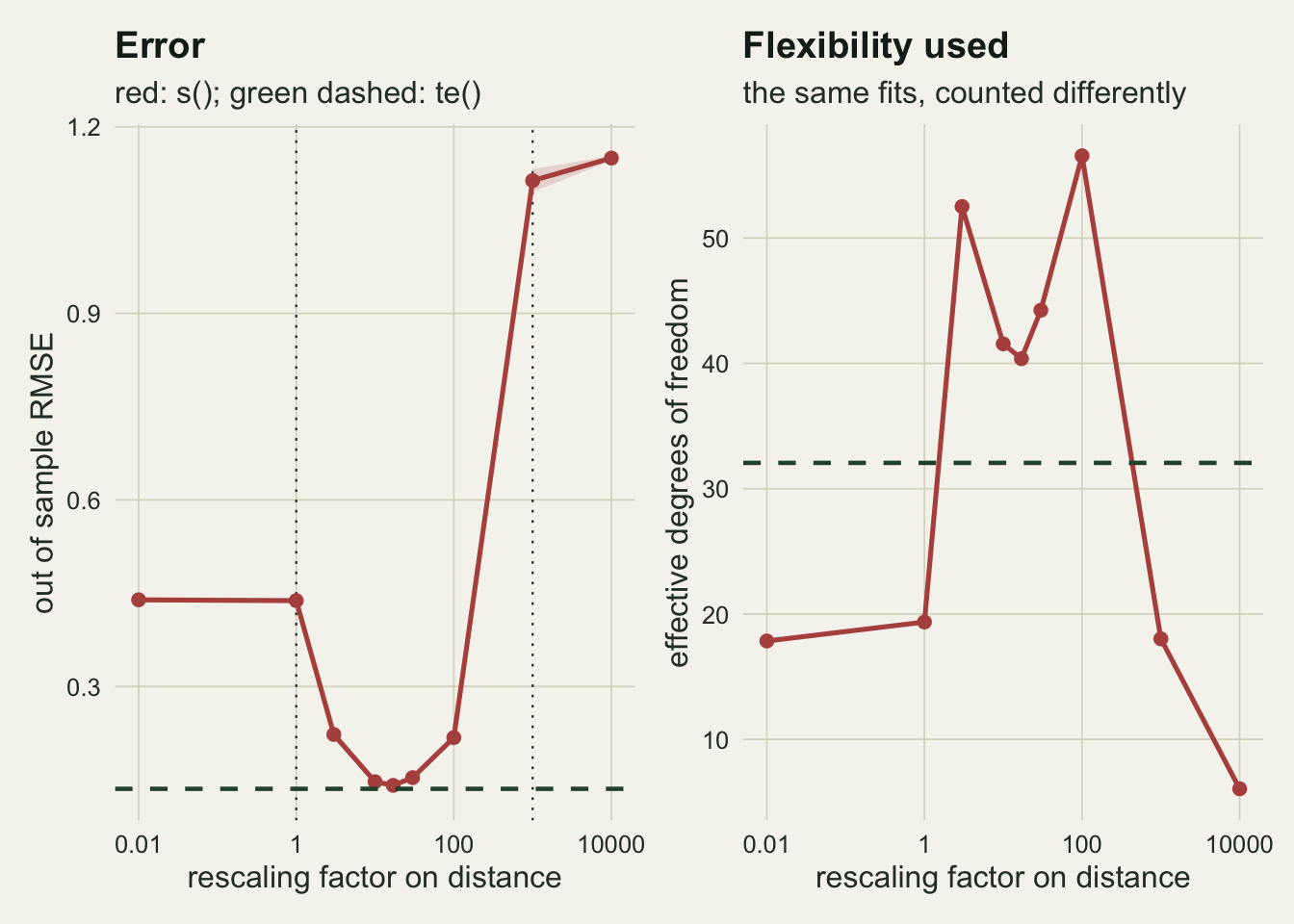
The tensor product line is flat because it has to be, which the next section takes apart. What is worth pausing on is the right panel. The effective degrees of freedom of the isotropic fit are not monotone in the rescaling: they run from 6.0 to 56.6 with the peak at a factor of 100, so a single before-and-after comparison can show the model getting either more flexible or less. A report that says the smooth used fewer degrees of freedom after a unit change has said nothing about whether the fit improved.
At the bottom of the U the two smoothers are close: the paired difference, isotropic minus tensor, is +0.0056 with a Monte Carlo standard error of 0.0043, which is 1.3 standard errors and therefore indistinguishable at 12 replicates. The gain from te() is not that it beats a well-rescaled isotropic smooth. It is that no rescaling had to be found.
te() removes the choice, and that is algebra
A tensor product smooth is built from one marginal basis per covariate, combined by taking products of the marginal basis functions, with one smoothing parameter per margin (Wood 2006). Three facts about that construction compose into an identity. The marginal bases are equivariant under an affine change of their own covariate: knots placed at quantiles, at evenly spaced points, or from within-margin distances all move with the data, so the space of functions the margin can represent is unchanged. The marginal penalties are normalised before they are combined, so the power of the scale factor that the penalty picks up is divided back out. And each marginal smoothing parameter is estimated freely, so any residual stretching is absorbed there. The consequence is not that te() is insensitive to units: it is that the fitted surface, its effective degrees of freedom and its REML score are the same objects before and after. The check below exists so a reader can confirm that on their own machine, not to establish it.
set.seed(2251)
one <- draw_survey()
fit_tensor <- function(mult, add, bases = c("cr", "cr")) {
  d <- one$tr; h <- one$ho
  d$xs <- one$tr$x * mult + add; h$xs <- one$ho$x * mult + add
  fit <- gam(y ~ te(xs, z, k = c(k_marg, k_marg), bs = bases),
             data = d, method = "REML")
  c(sqrt(mean((as.numeric(predict(fit, h)) - h$f)^2)),
    sum(fit$edf), unname(fit$gcv.ubre), unname(fit$sp[1]))
}

inv <- t(sapply(cs, function(cc) fit_tensor(1 / cc, 0)))
spread <- apply(inv[, 1:3], 2, function(v) max(abs(v - v[1])))
base_combo <- list(c("cr", "cr"), c("ps", "ps"), c("tp", "tp"), c("cr", "ps"))
affine     <- list(c(1e-3, 0), c(1e3, 0), c(1, -1000), c(2.7, 50))
aff <- do.call(rbind, lapply(base_combo, function(bb) {
  ref <- fit_tensor(1, 0, bb)
  t(sapply(affine, function(p) {
    v <- fit_tensor(p[1], p[2], bb)
    c(abs(v[1] - ref[1]), abs(v[2] - ref[2]), v[4] / ref[4])
  }))
}))
n_affine <- nrow(aff); max_drmse <- max(aff[, 1]); max_dedf <- max(aff[, 2])
sp_hi <- max(aff[, 3]); sp_dev <- max(abs(aff[, 3] - 1))
Refitting one dataset at every factor in the sweep moves the error by at most \(9.16 \times 10^{-16}\), the effective degrees of freedom by \(1.19 \times 10^{-12}\) and the REML score by \(1.31 \times 10^{-12}\): floating point and optimiser tolerances, not effects, and quoting a percentage change for them would be nonsense. Widening the check to affine maps, so a shift as well as a stretch, and to four combinations of marginal basis (cr with cr, ps with ps, tp with tp, and cr with ps), gives 16 refits whose largest error deviation is \(2.79 \times 10^{-14}\) and whose largest deviation in effective degrees of freedom is \(2.23 \times 10^{-11}\). The estimated smoothing parameter of the first margin comes back at a ratio of 1.000000 to its unscaled counterpart in every one of them, the largest deviation from unity being \(4.54 \times 10^{-13}\): not even the reported smoothing parameter moves.
The optimum tracks the anisotropy, not the noise
If the isotropic smooth needs a rescaling, it is fair to ask what the right one is. Setting the wiggliness per fitted unit equal on the two axes predicts a factor of the span ratio times the inverse ratio of cycles, span_x * wv / (span_z * wu), which is 16.7 for this seabed. The cells below vary the noise and the anisotropy of the truth to test that prediction; the sample size is held at 400 stills in every one of them, so nothing here speaks to how the optimum moves with n.
cs_cell <- c(1, 3, 10, 17, 30, 60, 100)
cell_rep <- 10; seed_cell <- 2253; big_k <- 12

cells <- data.frame(
  tag = c("noise sd 0.1", "baseline", "noise sd 1.5", "anisotropy 1", "anisotropy 6"),
  sd  = c(0.1, 0.5, 1.5, 0.5, 0.5), wu = c(1.5, 1.5, 1.5, 0.5, 3.0), wv = 0.5)
n_col <- length(cs_cell) + 2
cell_curve <- list(); cell_summ <- list(); arg_rep <- list()
for (i in seq_len(nrow(cells))) {
  ce <- cells[i, ]
  mat <- matrix(NA_real_, cell_rep, n_col)
  for (r in seq_len(cell_rep)) {
    set.seed(seed_cell + r)
    dd <- draw_survey(ce$wu, ce$wv, ce$sd); tr <- dd$tr; ho <- dd$ho
    for (j in seq_along(cs_cell)) {
      tr$xs <- tr$x / cs_cell[j]; ho$xs <- ho$x / cs_cell[j]
      mat[r, j] <- score_fit(y ~ s(xs, z, k = k_marg^2), tr, ho)[1]
    }
    tr$xs <- tr$x; ho$xs <- ho$x
    mat[r, n_col - 1] <- score_fit(y ~ te(xs, z, k = c(k_marg, k_marg)), tr, ho)[1]
    if (ce$tag == "anisotropy 6")
      mat[r, n_col] <- score_fit(y ~ te(xs, z, k = c(big_k, big_k)), tr, ho)[1]
  }
  swept <- mat[, seq_along(cs_cell)]; mu <- colMeans(swept); ranked <- order(mu)
  gap_r <- swept[, ranked[2]] - swept[, ranked[1]]
  arg_rep[[ce$tag]] <- apply(swept, 1, function(v) cs_cell[which.min(v)])
  cell_curve[[ce$tag]] <- data.frame(tag = ce$tag, cc = cs_cell, excess = mu / min(mu))
  cell_summ[[ce$tag]] <- data.frame(
    tag = ce$tag, aniso = ce$wu / ce$wv, star = span_x * ce$wv / (span_z * ce$wu),
    argmin = cs_cell[ranked[1]], best = min(mu), at_one = mu[1],
    depth = max(mu) / min(mu), ten = mean(mat[, n_col - 1]),
    ten_se = mc_se(mat[, n_col - 1]), margin_r = mean(gap_r),
    margin_se = mc_se(gap_r), margin_sigma = mean(gap_r) / mc_se(gap_r))
  if (ce$tag == "anisotropy 6") {
    te_big <- mean(mat[, n_col]); te_big_se <- mc_se(mat[, n_col])
    sharp_d <- mat[, n_col - 1] - mat[, 1]; big_d <- mat[, 1] - mat[, n_col]
    sharp_pair <- mean(sharp_d); sharp_pair_se <- mc_se(sharp_d)
    sharp_sigma <- sharp_pair / sharp_pair_se; sharp_lose <- sum(sharp_d > 0)
    big_pair <- mean(big_d); big_pair_se <- mc_se(big_d)
  }
}
cell_curve <- do.call(rbind, cell_curve)
cell_summ  <- do.call(rbind, cell_summ)
row.names(cell_summ) <- cell_summ$tag
arg_rep <- do.call(cbind, arg_rep)
deep <- cell_summ["noise sd 0.1", ]; shallow <- cell_summ["noise sd 1.5", ]
flat_cell <- cell_summ["anisotropy 1", ]; sharp_cell <- cell_summ["anisotropy 6", ]
sharp_wu <- cells$wu[cells$tag == "anisotropy 6"]; thin_i <- which.min(cell_summ$margin_sigma)
arg6 <- arg_rep[, "anisotropy 6"]; arg3 <- arg_rep[, "baseline"]; arg1 <- arg_rep[, "anisotropy 1"]
ord_hits <- sum(arg6 < arg1); ord_chain <- sum(arg6 < arg3 & arg3 < arg1)
ord_norev <- sum(arg6 <= arg3 & arg3 <= arg1); ord_tied <- ord_norev - ord_chain
thin_cell <- cell_summ[thin_i, ]
The minimum follows the truth’s anisotropy, not the noise. At an anisotropy of 1 the best factor on this grid is 60 against a prediction of 50.0; at 3 it is 17 against 16.7; at 6 it is 10 against 8.3, each on the grid point next to the closed form value. The shift is not an artefact of averaging replicates: the anisotropy of six cell puts its minimum to the left of the anisotropy of one cell in 10 of 10 replicates, on the same simulated surveys. That last cell is the one worth staring at: the truth there is equally wiggly across the two spans, and the optimal rescaling is still 60 rather than one, with error at metres of 0.5071 against 0.1088 at the optimum. Two covariates being in the same unit does not make them commensurate; the spans differ by a factor of 50, and the isotropic penalty sees only the raw numbers. Noise changes the depth of the U rather than its position: the three noise cells, whose standard deviations differ by a factor of 15, all put the minimum at the same 17. On the narrower grid used here, from a factor of one to a hundred, the worst to best ratio is 10.87 at the low noise setting and 1.64 at the high one. (These ratios come from a truncated grid and are not comparable with the sweep above, which runs four orders of magnitude wider.) Noise hides the geometry mistake; it does not repair it. The better the data, the more the choice of units is worth.
aniso_tags <- c("anisotropy 1", "baseline", "anisotropy 6")
noise_tags <- c("noise sd 0.1", "baseline", "noise sd 1.5")
pal3 <- c(te_forest, te_gold, te_rust)

panel_cell <- function(tags, labs_, leg, stars, ylab, ttl, sub_ttl) {
  d <- cell_curve[cell_curve$tag %in% tags, ]
  d$tag <- factor(d$tag, levels = tags, labels = labs_)
  lo <- do.call(rbind, lapply(split(d, d$tag), function(z) z[which.min(z$excess), ]))
  p <- ggplot(d, aes(cc, excess, colour = tag))
  if (stars) p <- p + geom_vline(
    data = data.frame(tag = factor(labs_, levels = labs_), star = cell_summ[tags, "star"]),
    aes(xintercept = star, colour = tag), linetype = "dotted",
    linewidth = 0.6, show.legend = FALSE)
  p + geom_line(linewidth = 0.9) +
    geom_point(data = lo, size = 3.2, colour = te_ink, show.legend = FALSE) +
    scale_colour_manual(values = pal3, name = leg, labels = labs_) + scale_x_log10() +
    labs(x = "rescaling factor", y = ylab, title = ttl, subtitle = sub_ttl) +
    theme_datasheet() + theme(legend.position = "bottom")
}

panel_cell(aniso_tags, c("1", "3 (baseline)", "6"), "anisotropy", TRUE,
           "RMSE relative to the curve's own best", "The truth moves the minimum",
           "dotted: predicted; dark dot: observed") +
  panel_cell(noise_tags, c("0.1", "0.5 (baseline)", "1.5"), "noise sd", FALSE,
             NULL, "The noise moves only the depth", "same minimum, different depth") +
  plot_annotation(theme = theme_datasheet())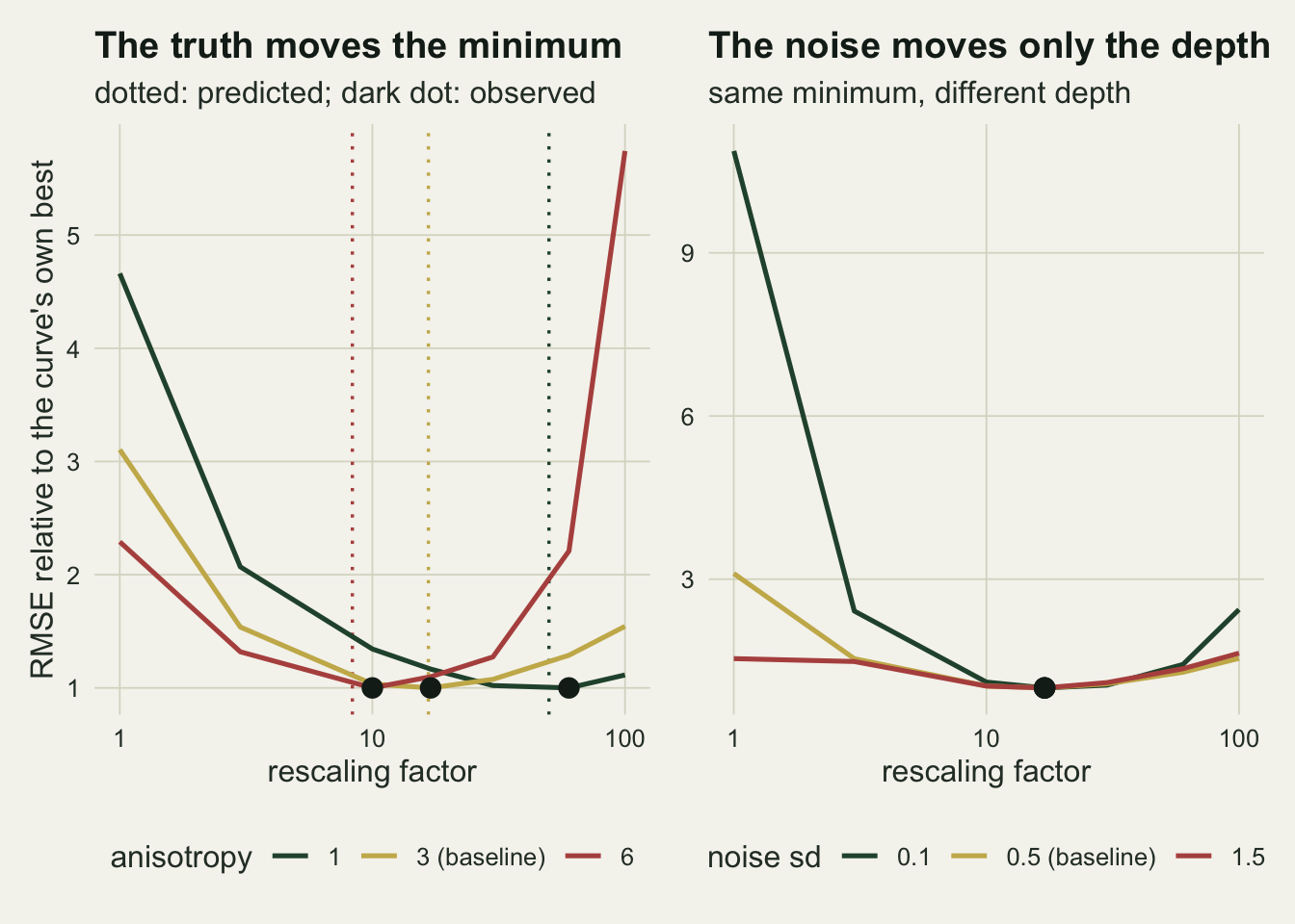
REML finds the rescaling, so the loss is recoverable
A tempting way to sell te() is to say the optimal rescaling is unknowable, since it depends on a truth nobody has. That is false, and the post would be worse for it. The restricted likelihood is a function of the fitted model alone, it needs no held-out data, and profiling it over the rescaling recovers the optimum (Wood 2011).
prof <- as.data.frame(t(sapply(seq_len(n_rep), function(r) {
  a <- sw[sw$rep == r, ]
  c(oracle_c = a$cc[which.min(a$s_rmse)], reml_c = a$cc[which.min(a$s_reml)],
    oracle = min(a$s_rmse), reml_pick = a$s_rmse[which.min(a$s_reml)])
})))

reml_hits <- sum(prof$reml_c == c_best); oracle_hits <- sum(prof$oracle_c == c_best)
agree_hits <- sum(prof$reml_c == prof$oracle_c); n_fits_needed <- length(cs)
oracle_rmse <- mean(prof$oracle);    oracle_se <- mc_se(prof$oracle)
picked_rmse <- mean(prof$reml_pick); picked_se <- mc_se(prof$reml_pick)
search_cost <- picked_rmse - oracle_rmse
The REML score picks the factor 17 in 12 of 12 replicates. The oracle, which is allowed to look at the held-out truth, picks the same factor in 9 of 12, and the two agree exactly in 9. Using the REML-chosen factor costs 0.1410 (standard error 0.0033) against 0.1406 (standard error 0.0033) for the oracle, a difference of 0.0004. So an ecologist who insists on s() is not doomed: they owe the reader a profile over a grid of factors, 9 of them here, a profile plot, and a sentence saying which rescaling was chosen and how. What te() saves is that step, plus the reporting burden that goes with it, and the tensor product still comes out at 0.1354 without any search at all.
When isotropy is true, the isotropic smoother wins
Everything above is a case where isotropy is false. Turn the design around: easting and northing of a plot grid, both in kilometres, and a truth built from radially symmetric bumps with the same length scale on both axes. There is no unit choice to make, and the isotropic penalty is now the correct prior belief about the surface rather than an accident of recording.
bumps <- function(x, y)
  1.8 * exp(-((x - 3)^2   + (y - 3)^2)   / (2 * 1.6^2)) -
  1.2 * exp(-((x - 7.5)^2 + (y - 6.5)^2) / (2 * 1.1^2)) +
  0.7 * exp(-((x - 6)^2   + (y - 2)^2)   / (2 * 0.9^2))

rev_rep <- 25; rev_sd <- 0.25; rev_span <- 10; seed_rev <- 2252
rev_out <- matrix(NA_real_, rev_rep, 4)
for (r in seq_len(rev_rep)) {
  set.seed(seed_rev + r)
  d <- data.frame(x = runif(n_train, 0, rev_span), y = runif(n_train, 0, rev_span))
  d$obs <- bumps(d$x, d$y) + rnorm(n_train, 0, rev_sd)
  h <- data.frame(x = runif(n_test, 0, rev_span), y = runif(n_test, 0, rev_span))
  h$f <- bumps(h$x, h$y)
  v_iso <- score_fit(obs ~ s(x, y, k = k_marg^2), d, h)
  v_ten <- score_fit(obs ~ te(x, y, k = c(k_marg, k_marg)), d, h)
  rev_out[r, ] <- c(v_iso[1], v_ten[1], v_iso[3], v_ten[3])
}
iso_rmse <- mean(rev_out[, 1]); iso_rmse_se <- mc_se(rev_out[, 1])
ten_iso <- mean(rev_out[, 2]); ten_iso_se <- mc_se(rev_out[, 2])
rev_d <- rev_out[, 2] - rev_out[, 1]; reml_d <- rev_out[, 4] - rev_out[, 3]
rev_pair <- mean(rev_d); rev_se <- mc_se(rev_d); rev_wins <- sum(rev_d > 0)
rev_cost <- 100 * (ten_iso / iso_rmse - 1); rev_sigma <- rev_pair / rev_se
reml_gap <- mean(reml_d); reml_gap_se <- mc_se(reml_d); reml_backs_te <- sum(reml_d < 0)
On this surface s(x, y) scores 0.0794 (standard error 0.0015) and te(x, y) scores 0.0834 (standard error 0.0015). The paired difference, tensor minus isotropic, is +0.0040 with a Monte Carlo standard error of 0.0006, and s() is the better fit in 22 of 25 replicates: a penalty of about 5 per cent for using the tensor product where isotropy holds.
panel_dec <- function(nm, mu, err, ylab, ttl, sub_ttl, note = NULL) {
  d <- data.frame(fit = factor(nm, levels = nm), rmse = mu, err = err,
                  kind = c(rep("isotropic smooth", length(nm) - 1), "tensor product"))
  p <- ggplot(d, aes(fit, rmse, colour = kind)) +
    geom_pointrange(aes(ymin = rmse - err, ymax = rmse + err), size = 0.7) +
    scale_colour_manual(values = c(te_rust, te_forest), name = NULL) +
    scale_y_continuous(expand = expansion(mult = 0.09)) +
    labs(x = NULL, y = ylab, title = ttl, subtitle = sub_ttl) +
    theme_datasheet() + theme(legend.position = "none")
  if (is.null(note)) return(p)
  top <- max(mu[-1]) + 0.06 * diff(range(mu))
  p + annotate("segment", x = 2, xend = 3, y = top, yend = top,
               colour = te_body, linewidth = 0.4) +
    annotate("text", x = 2.5, y = top, label = note, vjust = -0.6, size = 3.5,
             colour = te_body)
}

panel_dec(c("s() metres", "s() rescaled", "te()"),
          c(rmse_metres, rmse_bst, ten_rmse), c(agg$s_se[i_m], se_bst, ten_se),
          "out of sample RMSE", "Anisotropic truth",
          "transect metres against depth metres",
          note = sprintf("%.1f SE apart, not separated", opt_sigma)) +
  panel_dec(c("s()", "te()"), c(iso_rmse, ten_iso), c(iso_rmse_se, ten_iso_se),
            NULL, "Isotropic truth", "easting km against northing km") +
  plot_annotation(theme = theme_datasheet())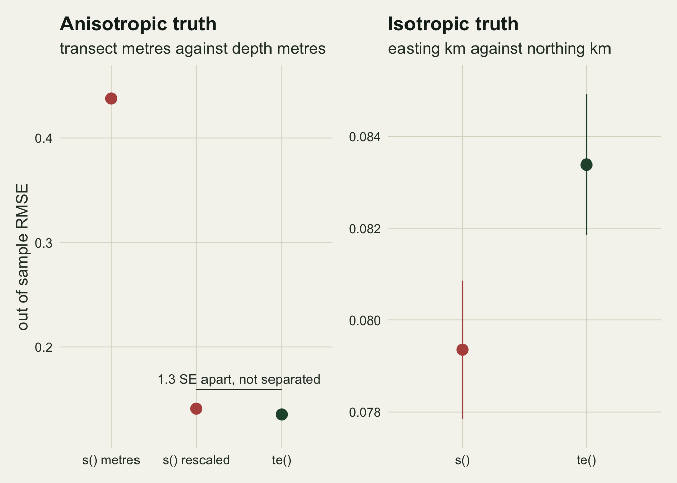
That is the shape of the decision. Getting the geometry wrong towards isotropy on this transect costs a factor of 3.24 at metres and 8.22 at kilometres. Getting it wrong towards the tensor product on a genuinely isotropic field costs 5 per cent. The asymmetry is the argument for a default, and the existence of a real cost is the argument for still thinking about it. One cost is still missing from that ledger: neither smoother above was fitted at the k that mgcv would pick for it. The chunk below leaves the isotropic plot grid, goes back to the seabed transect, and fits both smoothers at their defaults on further simulated surveys, with the tuned tensor product alongside on the same datasets. What it finds is a limit on the advice rather than a result about isotropy, so its numbers are read out under Honest limits.
def_rep <- 15; seed_def <- 2254
def_out <- matrix(NA_real_, def_rep, 5)
for (r in seq_len(def_rep)) {
  set.seed(seed_def + r)
  dd <- draw_survey(); tr <- dd$tr; ho <- dd$ho
  tr$xkm <- tr$x / 1000; ho$xkm <- ho$x / 1000
  def_out[r, ] <- c(score_fit(y ~ s(x, z),    tr, ho)[1],
                    score_fit(y ~ s(xkm, z),  tr, ho)[1],
                    score_fit(y ~ te(x, z),   tr, ho)[1],
                    score_fit(y ~ te(xkm, z), tr, ho)[1],
                    score_fit(y ~ te(x, z, k = c(k_marg, k_marg)), tr, ho)[1])
}
def_k <- gam(y ~ te(x, z), data = tr, method = "REML")$smooth[[1]]$margin[[1]]$bs.dim
def_s_m <- mean(def_out[, 1]); def_s_km <- mean(def_out[, 2])
def_ten <- mean(def_out[, 3]); def_ten_se <- mc_se(def_out[, 3])
def_ten8 <- mean(def_out[, 5]); def_ident <- max(abs(def_out[, 3] - def_out[, 4]))
def_s_d <- def_out[, 2] - def_out[, 1]; def_k_d <- def_out[, 3] - def_out[, 5]
def_pair <- mean(def_s_d); def_pair_se <- mc_se(def_s_d)
def_k_pair <- mean(def_k_d); def_k_se <- mc_se(def_k_d)
def_k_sigma <- def_k_pair / def_k_se; def_gap <- 100 * (def_ten / def_ten8 - 1)
def_kept <- 100 * (def_s_m - def_ten) / (def_s_m - def_ten8)
What to report
State the units of both covariates in a two-dimensional smooth, and say in one sentence whether the isotropic assumption is intended. A density surface model over projected coordinates in kilometres, as in Miller et al 2013, has every right to s(x, y), and saying so takes one clause. A smooth of distance against depth, or elevation against rainfall, needs a different sentence. If an isotropic smooth is used on covariates that are not commensurate, report the rescaling and how it was chosen: a REML profile over a grid of factors is cheap, needs no held-out data, and belongs in the supplement.
If a tensor product is used, report the basis dimension for each margin, not one number, and report what gam.check said about each margin separately: the margins are penalised separately, so they can run out of basis separately.
Do not compare REML scores between s() and te() and call the winner the better model: the scores come from different bases with different penalty null spaces, and the section below measures how badly that comparison misleads. Say which of the two smoothers was chosen before the data were seen, because the choice is a geometric claim about the field, and a claim made after looking at held-out error is a different kind of statement.
Honest limits
The tensor product’s default basis is small, and using it gives back about a quarter of what the tuned fit gained. te(x, z) defaults to 5 basis functions per margin. At the defaults the isotropic smooth scores 0.4398 in metres and 1.1591 in kilometres, a paired difference of +0.7194 with standard error 0.0077, while the default tensor product scores 0.2116 (standard error 0.0118) in both units, the two agreeing to within floating-point rounding. The default tensor product is still the best of the three, and on the same 15 surveys it retains 74 per cent of the distance between the default isotropic fit at metres and the tensor product with 8 per margin. What it gives up is +0.0786 (standard error 0.0113, 7.0 standard errors), or 59 per cent in relative terms. The advice that survives measurement is to use te() and set k per margin, then check both margins; the advice that does not survive is to use te() and stop thinking. What k is enough is the subject of the sibling post on basis dimension.
A tensor product can also lose its lead when a margin runs out of basis. In the anisotropy of six cell above, where the truth completes 3 cycles along the transect, te() at 8 per margin scores 0.4305 (standard error 0.0295) against 0.3914 for the isotropic fit at metres. Paired on the same 10 datasets that is +0.0391 with standard error 0.0293, 1.3 standard errors, with te() behind in 6 of 10: the mean is worse and the difference is not separated, which is enough to say the advantage seen elsewhere has gone. Raising both margins to 12 brings the same fit to 0.1718 (standard error 0.0045), ahead of metres by 0.2197 (standard error 0.0059) and level with the best isotropic rescaling in that cell, 0.1709. That last fit is no longer matched on basis size, 144 tensor coefficients against the 64 of s(), so it shows the margins were the binding constraint, not that te() wins at equal size.
The REML score is a poor compass for choosing between the two smoothers. On the isotropic surface, where s() predicts better by 6.4 standard errors, the tensor product has the lower REML score in 17 of 25 replicates, with a mean difference of -1.197 (standard error 0.528). The profile above stayed inside one family of bases: rescaling the covariate leaves the penalty null space the same set of functions, so the scores are comparable along that curve. s() and te() are different bases with different penalty null spaces, and that is the comparison the score cannot make. Pedersen et al 2019 make the same point for choices between hierarchical smoother structures.
The replication is deliberately small and it is not uniform: 12 replicates in the sweep, 10 per cell in the sensitivity grid, 25 in the isotropic reversal and 15 at the defaults. What that buys is uneven. The reversal’s 5 per cent penalty at 6.4 standard errors, the spread across the sweep, and the default-k gap at 7.0 are separated. Three comparisons are not: the isotropic and tensor fits at the bottom of the U differ by 1.3 standard errors, the same margin in the anisotropy of six cell is 1.3, and in the sensitivity grid the narrowest gap between a cell’s best factor and its runner-up is 1.2 standard errors (the anisotropy 1 cell, +0.0023 with standard error 0.0019). No single one of those minima is pinned down by its own margin; what carries that section is the ordering of the minima across the three anisotropy cells, and no replicate reverses it: the three fall weakly in order in 10 of 10, strictly in 8, and the remaining 2 put the anisotropy of six and the baseline minima on the same grid point, which at this grid spacing is a tie and not a reversal. Anyone wanting the margins sharpened should raise the replicate count rather than trust the sentence. The design is narrow in other ways as well: a Gaussian response, one sample size, independent uniform coverage of the covariate rectangle, matched basis sizes and a smooth deterministic truth. Not measured: Poisson or Tweedie counts, which is exactly what a density surface model fits; sampling constrained to transect lines, where coverage in one covariate is much better than in the other; covariates correlated with each other; and truths with sharp edges, where the marginal bases behave differently from either smoother’s assumption. The direction of the argument should carry, and the magnitudes should not be transferred to another design. Wood 2017 sets out the construction in full for anyone who wants the general case rather than this one.
References
Wood SN 2003 Journal of the Royal Statistical Society Series B 65(1):95-114 (10.1111/1467-9868.00374)
Wood SN 2006 Biometrics 62(4):1025-1036 (10.1111/j.1541-0420.2006.00574.x)
Wood SN 2011 Journal of the Royal Statistical Society Series B 73(1):3-36 (10.1111/j.1467-9868.2010.00749.x)
Wood SN 2017 Generalized Additive Models: An Introduction with R, 2nd edn (ISBN 978-1-4987-2833-1)
Miller DL, Burt ML, Rexstad EA, Thomas L 2013 Methods in Ecology and Evolution 4(11):1001-1010 (10.1111/2041-210X.12105)
Pedersen EJ, Miller DL, Simpson GL, Ross N 2019 PeerJ 7:e6876 (10.7717/peerj.6876)