library(ggplot2)
library(patchwork)
library(MASS)
library(mgcv)

te_paper  <- "#f5f4ee"
te_ink    <- "#16241d"
te_body   <- "#2c3a31"
te_forest <- "#275139"
te_rust   <- "#b5534e"
te_gold   <- "#c9b458"
te_line   <- "#dad9ca"

theme_datasheet <- function() {
  theme_minimal(base_size = 12) +
    theme(plot.background  = element_rect(fill = te_paper, colour = NA),
          panel.background = element_rect(fill = te_paper, colour = NA),
          panel.grid.major = element_line(colour = te_line, linewidth = 0.3),
          panel.grid.minor = element_blank(),
          text             = element_text(colour = te_body),
          plot.title       = element_text(colour = te_ink, face = "bold"),
          plot.subtitle    = element_text(colour = te_body),
          axis.text        = element_text(colour = te_body))
}Centring a quadratic before lasso or ridge
R
regression
regularisation
simulation
ecology tutorial
Standardising does not move the origin of a squared covariate. Simulating in R how lasso and ridge lose a thermal optimum on Celsius that centring keeps.
Sixty stream reaches along a temperature gradient from 2 to 22 C, one survey each, and an invertebrate whose abundance peaks somewhere in the middle. The thermal response is the question. Alongside temperature sit eight other reach covariates (substrate, shading, conductivity and the like), each allowed a linear and a squared term, because nobody knows in advance which of them bend. Eighteen columns against sixty rows is where this site sends people to a penalty: ridge regression or the lasso, with the columns standardised first. Temperature goes in as temp and temp^2, in Celsius, because that is how the logger reports it.
Least squares would not care. A quadratic in Celsius and a quadratic in temperature centred on its mean are the same family of curves, and the fitted curve, its optimum and every prediction are identical; the post on interaction terms makes the same point for products, that centring “only shifts where the intercept and main effects are evaluated”. A penalty is different. It prices coefficients, and where zero sits on the temperature axis decides what the hump costs. The post on collinearity and VIF says that centring the predictors before forming products “removes most of that artificial inflation” of the variance inflation factor; for least squares that is right, and under a penalty the same artefact changes the answer.
The closest relative on the site is the post on tensor product smooths, which showed that an isotropic smoothing penalty is not invariant to the unit of a covariate and that te() removes the choice. A penalty on a quadratic is not invariant to the origin either, and the site’s standing advice, standardise first, leaves the origin exactly where it was: only centring before squaring removes it. This is also not the problem in parameter scale and optim(), which is an optimiser stopping short. Every ridge and lasso fit below is exact (closed-form ridge, an exact lasso path), the REML fit is checked against a second implementation, and it is the penalised target itself that moves with the origin.
None of this is new as a principle. Peixoto 1987 set out why a polynomial model is invariant to a shift of origin only while its lower-order terms are kept, the well-formed or hierarchical rule, and Bien, Taylor and Tibshirani 2013 built a lasso that respects that hierarchy because the ordinary lasso does not. This post is a demonstration of those results in an ecological design, not a claim to them. The ridge half, and in particular what an estimated penalty does, is less often written down, and the measurements here are what the post adds: how often each penalty loses the hump, how early the damage sets in along the offset of the origin, what form the damage takes, and which repairs work.
One gradient, four origins
Each simulated dataset is one set of reaches. Temperature is uniform on 2 to 22 C with the optimum at 14 C, and the hump carries a fixed share of the response variance, R2_T. Three of the nuisance covariates have small linear effects carrying a share of 0.15; the rest of the eighteen columns carry nothing. The nuisance covariates are drawn with mean zero, so their own squares have no origin problem. The response is Gaussian.
The same data are then coded four ways. Only the origin of temperature changes, and it is summarised by the offset ratio, the mean of the variable that gets squared divided by its standard deviation. Centred temperature has a ratio of 0. Celsius on 2 to 22 C has a ratio of 12 over the standard deviation of that uniform. A ratio of 4 stands in for the covariates recorded far from zero, such as day of year or rainfall in millimetres, and kelvin sits at the far end. Each coding is built from the sample: temperature minus its sample mean plus the ratio times its sample standard deviation, so the Celsius and kelvin codings are Celsius and kelvin up to sampling noise in that mean and standard deviation.
t_lo <- 2; t_hi <- 22; t_opt <- 14      # temperature range and optimum, C
p_nuis <- 8; share_nuis <- 0.15         # nuisance covariates and their variance share
w_nuis <- c(0.4, -0.3, 0.2)             # weights of the three nuisance covariates with an effect
n_ds <- 100                             # datasets per cell, fixed before any rate was seen
sd_unif <- (t_hi - t_lo) / sqrt(12)
ratio_celsius <- ((t_lo + t_hi) / 2) / sd_unif
ratio_kelvin  <- ((t_lo + t_hi) / 2 + 273.15) / sd_unif
codings <- c(centred = 0, celsius = ratio_celsius, ratio4 = 4, kelvin = ratio_kelvin)
coding_lab <- c(centred = "centred", celsius = "Celsius", ratio4 = "ratio 4", kelvin = "kelvin")

make_sites <- function(n, r2_t) {
  temp <- runif(n, t_lo, t_hi)
  nuis <- matrix(rnorm(n * p_nuis), n)
  nuis2 <- scale(nuis^2, scale = FALSE)
  hump <- -(temp - t_opt)^2; hump_sd <- sd(hump)
  lin <- as.numeric(nuis[, 1:3] %*% w_nuis); lin <- lin / sd(lin)
  y <- sqrt(r2_t) * (hump - mean(hump)) / hump_sd + sqrt(share_nuis) * lin +
       rnorm(n, 0, sqrt(1 - r2_t - share_nuis))
  t_grid <- seq(quantile(temp, 0.05), quantile(temp, 0.95), length.out = 50)
  truth <- sqrt(r2_t) * (-(t_grid - t_opt)^2) / hump_sd
  list(temp = temp, nuis = nuis, nuis2 = nuis2, y = y, r2_t = r2_t,
       t_grid = t_grid, truth = truth - mean(truth),
       fine = seq(min(temp), max(temp), length.out = 2001),
       folds = sample(rep(1:5, length.out = n)))
}
coded_design <- function(s, ratio) {
  u <- s$temp - mean(s$temp) + ratio * sd(s$temp)
  cbind(u = u, u2 = u^2, s$nuis, s$nuis2)
}
Standardising a column subtracts its mean and divides by its standard deviation, and neither step touches a correlation. So whatever correlation temperature has with its own square survives standardisation untouched. For a uniform variable with offset ratio r that correlation has a closed form: writing the variable as r plus a standardised uniform z, the covariance with its square is 2r and the variance of the square is 4r^2 plus the variance of z^2, which is 0.8 for a uniform, so the correlation is r divided by the square root of r^2 plus 0.2.
corr_closed <- function(r) r / sqrt(r^2 + 0.2)
set.seed(3270)
chk_sites <- make_sites(60, 0.1)
corr_sample <- sapply(codings, function(r) { X <- coded_design(chk_sites, r); cor(X[, 1], X[, 2]) })
corr_theory <- corr_closed(codings)
The closed form gives 0.978 for Celsius, 0.994 at a ratio of 4 and 0.99996 in kelvin, against 0.979, 0.995 and 0.99997 in one simulated set of sixty reaches. That correlation is arithmetic, and it is the anchor for what follows, not the finding.
Four ways to fit, all exact
The fits are written out in base R so that nothing in them is an approximation that could depend on the coding. Every penalty acts on standardised columns, with the intercept left out, which is the convention of the ridge and lasso posts and of glmnet. Ridge (Hoerl and Kennard 1970) on a grid of penalties is one singular value decomposition, and generalised cross-validation (GCV) picks the penalty with the same criterion MASS::lm.ridge uses. The lasso path is computed exactly by least angle regression with the lasso modification, which is piecewise linear in the penalty, and five-fold cross-validation picks the minimum. The third penalised fit is ridge with one shared prior variance for all eighteen slopes, estimated by restricted maximum likelihood (REML) through mgcv; the fourth is a fixed prior, kept apart from it on purpose.
standardise_cols <- function(X) {
  ctr <- colMeans(X); Xc <- sweep(X, 2, ctr)
  scl <- sqrt(colMeans(Xc^2))                 # n divisor, as lm.ridge and glmnet
  list(Z = sweep(Xc, 2, scl, "/"), ctr = ctr, scl = scl)
}
to_raw_scale <- function(b_std, st, ybar) {   # standardised slopes -> intercept + raw slopes
  b_raw <- as.matrix(b_std) / st$scl
  rbind(ybar - colSums(b_raw * st$ctr), b_raw)
}
# ridge on a grid: minimise ||yc - Z b||^2 + lambda ||b||^2, one SVD for the whole grid
ridge_svd <- function(Z, yc, lambdas, sv = svd(Z)) {
  uy <- as.numeric(crossprod(sv$u, yc)); dd <- sv$d
  B <- sv$v %*% (outer(dd, lambdas, function(a, l) a / (a^2 + l)) * uy)
  df_eff <- colSums(outer(dd^2, lambdas, function(a, l) a / (a + l)))
  list(B = B, df = df_eff, rss = colSums((yc - Z %*% B)^2))
}
fit_ridge_gcv <- function(X, y, lambdas = 10^seq(-4, 4, length.out = 81)) {
  st <- standardise_cols(X); rp <- ridge_svd(st$Z, y - mean(y), lambdas)
  k <- which.min(rp$rss / (nrow(X) - rp$df)^2)
  list(coef = to_raw_scale(rp$B[, k], st, mean(y))[, 1], lambda = lambdas[k])
}
# exact lasso path: minimise (1 / 2n) ||yc - Z b||^2 + lam ||b||_1
lasso_path <- function(Z, yc, eps = 1e-12) {
  n <- nrow(Z); p <- ncol(Z); b <- numeric(p); mu <- numeric(n)
  cr0 <- as.numeric(crossprod(Z, yc)); active <- which.max(abs(cr0))
  lam <- max(abs(cr0)) / n; B <- matrix(0, p, 1)
  for (step in seq_len(4 * p)) {
    cr <- as.numeric(crossprod(Z, yc - mu)); cmax <- max(abs(cr[active]))
    sg <- sign(cr[active]); ZA <- sweep(Z[, active, drop = FALSE], 2, sg, "*")
    g1 <- as.numeric(solve(crossprod(ZA), rep(1, length(active))))
    aa <- 1 / sqrt(sum(g1)); w <- aa * g1
    u <- as.numeric(ZA %*% w); a <- as.numeric(crossprod(Z, u))
    idle <- setdiff(seq_len(p), active); j_in <- NA; gam <- cmax / aa
    if (length(idle)) {
      gp <- (cmax - cr[idle]) / (aa - a[idle]); gm <- (cmax + cr[idle]) / (aa + a[idle])
      gg <- pmin(ifelse(gp > eps, gp, Inf), ifelse(gm > eps, gm, Inf))
      if (min(gg) < gam) { gam <- min(gg); j_in <- idle[which.min(gg)] }
    }
    dirn <- sg * w; hit0 <- -b[active] / dirn; hit0[hit0 <= eps] <- Inf; j_out <- NA
    if (min(hit0) < gam) { gam <- min(hit0); j_out <- active[which.min(hit0)]; j_in <- NA }
    b[active] <- b[active] + gam * dirn; mu <- mu + gam * u; cmax <- cmax - gam * aa
    if (!is.na(j_out)) { b[j_out] <- 0; active <- setdiff(active, j_out) }
    if (!is.na(j_in)) active <- c(active, j_in)
    lam <- c(lam, max(cmax, 0) / n); B <- cbind(B, b)
    if (cmax <= 1e-10 * lam[1] * n || (is.na(j_in) && is.na(j_out))) break
  }
  list(lam = lam, B = B)
}
lasso_at <- function(path, lam_out) {         # linear interpolation along the exact path
  L <- path$lam; lam_out <- pmin(pmax(lam_out, min(L)), max(L))
  k <- pmin(pmax(findInterval(-lam_out, -L, rightmost.closed = TRUE), 1), length(L) - 1)
  wt <- (lam_out - L[k]) / (L[k + 1] - L[k]); wt[!is.finite(wt)] <- 0
  path$B[, k, drop = FALSE] + sweep(path$B[, k + 1, drop = FALSE] - path$B[, k, drop = FALSE], 2, wt, "*")
}
fit_lasso_cv <- function(X, y, folds, n_lam = 40) {
  st <- standardise_cols(X); full <- lasso_path(st$Z, y - mean(y))
  lams <- full$lam[1] * 10^seq(0, -3, length.out = n_lam)
  cv_err <- matrix(0, max(folds), n_lam)
  for (k in seq_len(max(folds))) {
    tr <- folds != k; s_k <- standardise_cols(X[tr, , drop = FALSE])
    B_k <- to_raw_scale(lasso_at(lasso_path(s_k$Z, y[tr] - mean(y[tr])), lams), s_k, mean(y[tr]))
    cv_err[k, ] <- colMeans((y[!tr] - cbind(1, X[!tr, , drop = FALSE]) %*% B_k)^2)
  }
  best <- which.min(colMeans(cv_err))
  list(coef = to_raw_scale(lasso_at(full, lams[best]), st, mean(y))[, 1], lambda = lams[best],
       at_floor = best == n_lam)
}
# ridge with one shared prior variance, estimated by REML in mgcv
fit_ridge_reml <- function(X, y) {
  st <- standardise_cols(X); Z <- st$Z
  g <- gam(y ~ Z, paraPen = list(Z = list(diag(ncol(Z)))), method = "REML")
  b <- coef(g)
  list(coef = c(b[1] - sum(b[-1] / st$scl * st$ctr), b[-1] / st$scl), lambda = unname(g$sp[1]))
}
# a fixed prior: normal(0, (2.5 sd(y))^2) on every standardised slope, joint mode with sigma
fit_ridge_fixed <- function(X, y, prior_sd = 2.5 * sd(y)) {
  st <- standardise_cols(X); yc <- y - mean(y); sv <- svd(st$Z); s2 <- var(y)
  for (it in 1:500) {
    rp <- ridge_svd(st$Z, yc, s2 / prior_sd^2, sv)
    if (abs(rp$rss / nrow(X) - s2) < 1e-12) break
    s2 <- rp$rss / nrow(X)
  }
  list(coef = to_raw_scale(rp$B[, 1], st, mean(y))[, 1], lambda = s2 / prior_sd^2)
}
Two of these deserve a check against an outside reference before anything is measured with them. The GCV ridge should reproduce MASS::lm.ridge exactly, and the lasso path should reproduce plain coordinate descent, the algorithm the lasso post codes, at any penalty on the path. Coordinate descent is run once only, on one dataset, as an outside check on the path.
X_chk <- coded_design(chk_sites, ratio_celsius); y_chk <- chk_sites$y
lr <- lm.ridge(y_chk ~ X_chk, lambda = 10^seq(-4, 4, length.out = 81))
gap_gcv <- max(abs(coef(lr)[which.min(lr$GCV), ] - fit_ridge_gcv(X_chk, y_chk)$coef))

st_chk <- standardise_cols(X_chk); yc_chk <- y_chk - mean(y_chk)
path_chk <- lasso_path(st_chk$Z, yc_chk); lam_chk <- 0.05 * path_chk$lam[1]
soft <- function(z, g) sign(z) * pmax(abs(z) - g, 0)
b_cd <- numeric(ncol(X_chk)); res_cd <- yc_chk
for (sweep_no in 1:100000) {
  b_old <- b_cd
  for (j in seq_along(b_cd)) {
    res_cd <- res_cd + st_chk$Z[, j] * b_cd[j]
    b_cd[j] <- soft(sum(st_chk$Z[, j] * res_cd) / nrow(X_chk), lam_chk)
    res_cd <- res_cd - st_chk$Z[, j] * b_cd[j]
  }
  if (max(abs(b_cd - b_old)) < 1e-13) break
}
gap_lars <- max(abs(lasso_at(path_chk, lam_chk)[, 1] - b_cd))
On the Celsius coding of the check dataset the GCV ridge matches lm.ridge to within floating-point rounding and the lasso path matches coordinate descent to \(4.5 \times 10^{-14}\), after 39 coordinate descent sweeps. The REML ridge gets its own, stricter check further down, because its result is the most extreme in the post.
Least squares does not care where zero is
The main experiment crosses two sample sizes, 60 and 150 reaches, with two hump shares, R2_T of 0.1 and 0.3, and fits every coding of every dataset with least squares, GCV ridge, the cross-validated lasso and REML ridge. The five folds are drawn once per dataset and shared by all codings, so the codings are compared on identical splits. A dataset counts as having found the hump when the fitted temperature curve has its maximum strictly inside the observed range, which for a quadratic is the same as a negative squared coefficient with the vertex inside the data; a curve that varies by less than \(10^{-4}\) response standard deviations across the whole range counts as flat, not as a hump. The curve error is the root mean square difference from the true curve over fifty temperatures between the 5 and 95 per cent quantiles of the observed range, in standard deviations of the true curve. The optimum error is measured only on fits that found a hump.
score_curve <- function(curve_fn, s) {
  cf <- curve_fn(s$fine); k <- which.max(cf)
  found <- k > 1 && k < length(cf) && diff(range(cf)) > 1e-4   # a flat curve is no hump
  cg <- curve_fn(s$t_grid)
  c(hump = found, opt_err = if (found) s$fine[k] - t_opt else NA,
    rmse = sqrt(mean((cg - mean(cg) - s$truth)^2)) / sqrt(s$r2_t))
}
quad_curve <- function(b, s, ratio) {
  b <- unname(b); shift <- ratio * sd(s$temp) - mean(s$temp)
  function(tt) b[2] * (tt + shift) + b[3] * (tt + shift)^2
}
fit_coded <- function(s, ratio, method) {
  X <- coded_design(s, ratio); y <- s$y
  f <- switch(method,
              ols   = list(coef = coef(lm(y ~ X)), lambda = 0),
              gcv   = fit_ridge_gcv(X, y),
              lasso = fit_lasso_cv(X, y, s$folds),
              reml  = fit_ridge_reml(X, y),
              fixed = fit_ridge_fixed(X, y))
  b <- unname(f$coef)
  c(score_curve(quad_curve(b, s, ratio), s), lambda = f$lambda, b_u = b[2], b_u2 = b[3],
    at_floor = if (is.null(f$at_floor)) NA else f$at_floor)
}
cells <- expand.grid(n = c(60, 150), r2_t = c(0.1, 0.3))
main_methods <- c("ols", "gcv", "lasso", "reml", "fixed")
anchor_sites <- list()
set.seed(3271)
main_rows <- list(); ols_gaps <- numeric(0)
for (i in seq_len(nrow(cells))) for (d in seq_len(n_ds)) {
s <- make_sites(cells$n[i], cells$r2_t[i])
if (cells$n[i] == 60 && cells$r2_t[i] == 0.1) anchor_sites[[d]] <- s
ols_vals <- sapply(codings, function(r) fitted(lm(s$y ~ coded_design(s, r))))
ols_gaps <- c(ols_gaps, max(abs(ols_vals - ols_vals[, 1])))
for (cn in names(codings)) for (m in main_methods)
main_rows[[length(main_rows) + 1]] <- c(cell = i, ds = d, fit_coded(s, codings[[cn]], m),
coding = match(cn, names(codings)),
method = match(m, main_methods))
}
main_res <- as.data.frame(do.call(rbind, main_rows))
main_res$coding <- names(codings)[main_res$coding]
main_res$method <- main_methods[main_res$method]
main_res$n <- cells$n[main_res$cell]; main_res$r2_t <- cells$r2_t[main_res$cell]
ols_gap <- max(ols_gaps)
share_of <- function(m, cn, nn = 60, rr = 0.1, what = "hump")
mean(main_res[[what]][main_res$method == m & main_res$coding == cn & main_res$n == nn & main_res$r2_t == rr])
paired_se <- function(m, nn = 60, rr = 0.1) {
a <- main_res$hump[main_res$method == m & main_res$coding == "centred" & main_res$n == nn & main_res$r2_t == rr]
b <- main_res$hump[main_res$method == m & main_res$coding == "celsius" & main_res$n == nn & main_res$r2_t == rr]
sd(a - b) / sqrt(length(a))
}
mcse_half <- sqrt(0.25 / n_ds)
gcv_rows <- main_res$method == "gcv"
la_rows <- main_res$method == "lasso"
lasso_floor <- mean(main_res$at_floor[la_rows])
lasso_floor_hump <- mean(main_res$hump[la_rows & main_res$at_floor == 1])
gcv_top <- main_res$lambda[gcv_rows] >= 1e4 * 0.9999
gcv_top_share <- mean(gcv_top); gcv_bottom_share <- mean(main_res$lambda[gcv_rows] <= 1e-4 * 1.0001)
gcv_top_hump <- mean(main_res$hump[gcv_rows][gcv_top])Least squares is the control, and it passes exactly. Across all 400 datasets the fitted values differ between the four codings by at most \(3.0 \times 10^{-11}\) response units, so every least squares number below is one number, not four. At 60 reaches and R2_T of 0.1, least squares finds the hump in 94 per cent of datasets in every coding.
The penalty does care
h_lasso_c <- share_of("lasso", "centred"); h_lasso_k <- share_of("lasso", "celsius")
h_gcv_c <- share_of("gcv", "centred");     h_gcv_k <- share_of("gcv", "celsius")
se_lasso <- paired_se("lasso"); se_gcv <- paired_se("gcv")
cell_tab <- aggregate(hump ~ n + r2_t + method + coding, main_res, mean)
strong_min <- min(cell_tab$hump[cell_tab$n == 150 & cell_tab$r2_t == 0.3 & cell_tab$method %in% c("gcv", "lasso")])
la_head <- main_res[main_res$method == "lasso" & main_res$coding == "centred" & main_res$n == 60 & main_res$r2_t == 0.1, ]
n_hump_head <- sum(la_head$hump)
n_pinned_head <- sum(la_head$hump == 1 & la_head$b_u == 0 & la_head$b_u2 != 0)   # linear term dropped
reml_unc_max <- max(cell_tab$hump[cell_tab$method == "reml" & cell_tab$coding != "centred"])
With 60 reaches and a thermal signal carrying a tenth of the variance, least squares finds the hump in 94 per cent of datasets whatever the units; the cross-validated lasso returns a hump in 61 per cent after centring and 4 per cent on plain Celsius. In 27 of those 61 centred humps the lasso dropped the linear term, so the vertex is simply the sample mean; the section on repairs comes back to them. GCV ridge goes from 93 to 16 per cent. The standard errors of those paired differences are 0.050 and 0.042, against a Monte Carlo standard error of at most 0.050 for any single share out of 100 datasets.
The same data, the same folds, the same penalty family; the only thing that changed is which temperature was called zero before squaring. Standardising was applied in both codings, as the ridge and lasso posts prescribe, and it did not help.
meth_lab <- c(ols = "least squares", gcv = "GCV ridge", lasso = "CV lasso", reml = "REML ridge", fixed = "fixed prior")
meth_col <- c("least squares" = te_ink, "GCV ridge" = te_forest, "CV lasso" = te_rust,
              "REML ridge" = te_gold, "fixed prior" = "#8a8f7a")
gt <- cell_tab[cell_tab$method != "fixed", ]
gt$fit <- factor(meth_lab[gt$method], levels = meth_lab[1:4])
gt$coding <- factor(coding_lab[gt$coding], levels = coding_lab)
gt$panel <- factor(sprintf("n = %d, R2_T = %.1f", gt$n, gt$r2_t),
                   levels = sprintf("n = %d, R2_T = %.1f", c(60, 150, 60, 150), c(0.1, 0.1, 0.3, 0.3)))
gt$mcse <- sqrt(gt$hump * (1 - gt$hump) / n_ds)
ggplot(gt, aes(coding, hump, colour = fit, group = fit)) +
  geom_errorbar(aes(ymin = pmax(hump - 2 * mcse, 0), ymax = pmin(hump + 2 * mcse, 1)),
                width = 0.15, linewidth = 0.4, position = position_dodge(width = 0.35)) +
  geom_line(linewidth = 0.8, position = position_dodge(width = 0.35)) +
  geom_point(size = 2, position = position_dodge(width = 0.35)) +
  facet_wrap(~panel, ncol = 2) +
  scale_colour_manual(values = meth_col, name = NULL) +
  scale_y_continuous(limits = c(0, 1)) +
  labs(x = "coding of temperature before squaring", y = "share of datasets with a hump inside the data",
       title = "Only least squares ignores the origin",
       subtitle = "same datasets in every coding; columns standardised before every penalty") +
  theme_datasheet() + theme(legend.position = "bottom")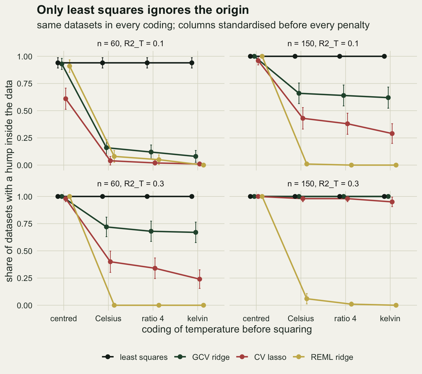
The damage shrinks as the penalty has less to do. At 150 reaches and R2_T of 0.3 the lowest hump share for GCV ridge or the lasso in any coding is 0.95, so with a strong signal and plenty of sites the two data-tuned penalties barely notice the origin. REML ridge is the exception: in no panel does any uncentred coding reach a hump share above 0.08, and it has its own section below.
Why standardising leaves the origin in place
The mechanism is visible in the coefficients the hump needs. In standardised units the true curve is a combination of standardised temperature and standardised squared temperature, and how large those two coefficients must be depends only on the offset ratio. With the temperature written as r plus a standardised uniform z and the optimum at z0 on that scale, the hump is minus z squared plus 2 z0 z, which is minus the squared column plus (2r + 2 z0) times the linear column plus a constant. Dividing each by its standard deviation gives the standardised coefficients in closed form, and their sizes are what the penalties price: ridge charges the squared length, the lasso the sum of absolute values.
z_opt <- (t_opt - (t_lo + t_hi) / 2) / sd_unif
hump_price <- function(r, r2_t = 0.1) {
  k_scale <- sqrt(r2_t) / sqrt(0.8 + 4 * z_opt^2)          # sets the hump variance to r2_t
  b_sq <- -k_scale * sqrt(4 * r^2 + 0.8); b_lin <- k_scale * (2 * r + 2 * z_opt)
  c(l2 = sqrt(b_sq^2 + b_lin^2), l1 = abs(b_sq) + abs(b_lin), b_lin = b_lin, b_sq = b_sq)
}
price_tab <- sapply(codings, hump_price)
eig_small <- function(r, n = 60) n * (1 - corr_closed(r))    # small eigenvalue of the (u, u2) pair
lam_med <- function(m, cn) median(main_res$lambda[main_res$method == m & main_res$coding == cn &
                                                  main_res$n == 60 & main_res$r2_t == 0.1])
shrink_at <- function(m, cn) eig_small(codings[[cn]]) / (eig_small(codings[[cn]]) + lam_med(m, cn))
Centred, the hump needs standardised coefficients of total length 0.32 response standard deviations. In Celsius it needs +1.36 on the linear column and -1.19 on the squared one, two large coefficients of opposite sign whose length is 1.80; in kelvin the length is 39.2. The curve is the same in every case. What changes is that in an uncentred coding the hump can only be written as the small difference of two large, nearly collinear terms, and a penalty charges for the terms, not for the difference.
Ridge sees the same thing through the eigenvalues of the standardised design. Two standardised columns correlated at rho have eigenvalues n(1 + rho) and n(1 - rho), and in an uncentred coding the hump lies almost entirely along the second, the direction in which the two coefficients move in opposite senses. Ridge multiplies each eigen-direction by its eigenvalue over the eigenvalue plus the penalty. At 60 reaches that smallest eigenvalue is 60.0 centred and 1.34 in Celsius. The median penalty GCV chose was 50.1 centred and 79.4 in Celsius, so the hump direction keeps roughly a fraction 0.54 of its least squares size when centred and 0.02 in Celsius. The lasso cannot buy the hump at all without paying for both large coefficients, and a line through the data, one coefficient and no curvature, is usually cheaper.
extra_ratios <- c(r05 = 0.5, r1 = 1, maxent = 0.5 / sqrt(1 / 12), r10 = 10, r20 = 20)
off_methods <- c("gcv", "lasso", "reml", "fixed")
off_rows <- list()
for (d in seq_len(n_ds)) for (cn in names(extra_ratios)) for (m in off_methods)
  off_rows[[length(off_rows) + 1]] <- c(ratio = extra_ratios[[cn]], method = match(m, off_methods),
                                        fit_coded(anchor_sites[[d]], extra_ratios[[cn]], m)[c("hump", "rmse")])
off_res <- as.data.frame(do.call(rbind, off_rows))
off_res$method <- off_methods[off_res$method]
anchor_main <- main_res[main_res$n == 60 & main_res$r2_t == 0.1 & main_res$method %in% off_methods,
                        c("coding", "method", "hump", "rmse")]
anchor_main$ratio <- codings[anchor_main$coding]
off_all <- rbind(off_res, anchor_main[, c("ratio", "method", "hump", "rmse")])
off_tab <- aggregate(cbind(hump, rmse) ~ ratio + method, off_all, mean)
off_at <- function(m, r) off_tab$hump[off_tab$method == m & abs(off_tab$ratio - r) < 1e-9]
The damage also starts early. Refitting the anchor datasets at offset ratios of 0.5 and 1, GCV ridge finds the hump in 66 and 38 per cent of them and the lasso in 31 and 9 per cent. From Celsius onwards the shares for the tuned penalties fall only slowly: refitted also at ratios of 10 and 20, GCV ridge reads 0.16, 0.12, 0.10, 0.08 and 0.08 at Celsius, ratios of 4, 10 and 20, and kelvin, even though the price of the hump keeps climbing by more than an order of magnitude. Once the hump costs more than the penalty will pay, the fit switches to a line, and a more expensive hump is dropped in the same way.
MaxEnt is the case worth naming. It rescales each covariate to the unit interval before squaring, which puts the origin at the data minimum; for a uniform covariate that is an offset ratio of 0.5 over the standard deviation of a unit uniform, 1.73. Its per-feature regularisation is proportional to the standard deviation of each feature, as the MaxEnt post codes it, which is the same thing as standardising before a common penalty. So its quadratic features sit in the uncentred regime: at that ratio GCV ridge here finds the hump in 19 per cent of datasets and the lasso in 4 per cent. MaxEnt’s own loss and its hinge features were not simulated here.
ot <- off_tab; ot$fit <- factor(meth_lab[ot$method], levels = meth_lab[c(2, 3, 4, 5)])
r_breaks <- c(0, 0.5, 1, ratio_celsius, 4, 10, 20, ratio_kelvin); r_labs <- sprintf("%g", round(r_breaks, 2))
p_off <- ggplot(ot, aes(1 + ratio, hump, colour = fit)) +
  geom_line(linewidth = 0.8) + geom_point(size = 2) +
  scale_x_log10(breaks = 1 + r_breaks, labels = r_labs) +
  scale_y_continuous(limits = c(0, 1)) +
  scale_colour_manual(values = meth_col, name = NULL) +
  guides(colour = guide_legend(nrow = 2)) +
  labs(x = "offset ratio (log scale of 1 + ratio)", y = "share of datasets with a hump",
       title = "Tuned penalties drop the hump early", subtitle = "same 100 datasets at every ratio") +
  theme_datasheet() + theme(legend.position = "bottom")
r_seq <- c(0, 10^seq(-1.5, log10(60), length.out = 80))
pr <- data.frame(ratio = rep(r_seq, 2),
                 price = c(sapply(r_seq, function(r) hump_price(r)["l2"]), sapply(r_seq, function(r) hump_price(r)["l1"])),
                 norm = rep(c("length (ridge norm)", "absolute sum (lasso norm)"), each = length(r_seq)))
p_price <- ggplot(pr, aes(1 + ratio, price, linetype = norm)) +
  geom_line(colour = te_ink, linewidth = 0.8) +
  scale_x_log10(breaks = 1 + r_breaks, labels = r_labs) + scale_y_log10() +
  scale_linetype_manual(values = c("solid", "22"), name = NULL) +
  guides(linetype = guide_legend(nrow = 2)) +
  labs(x = "offset ratio (log scale of 1 + ratio)", y = "size of the needed coefficients",
       title = "The price of the same hump", subtitle = "closed form, in response SDs") +
  theme_datasheet() + theme(legend.position = "bottom")
p_off + p_price + plot_annotation(theme = theme_datasheet())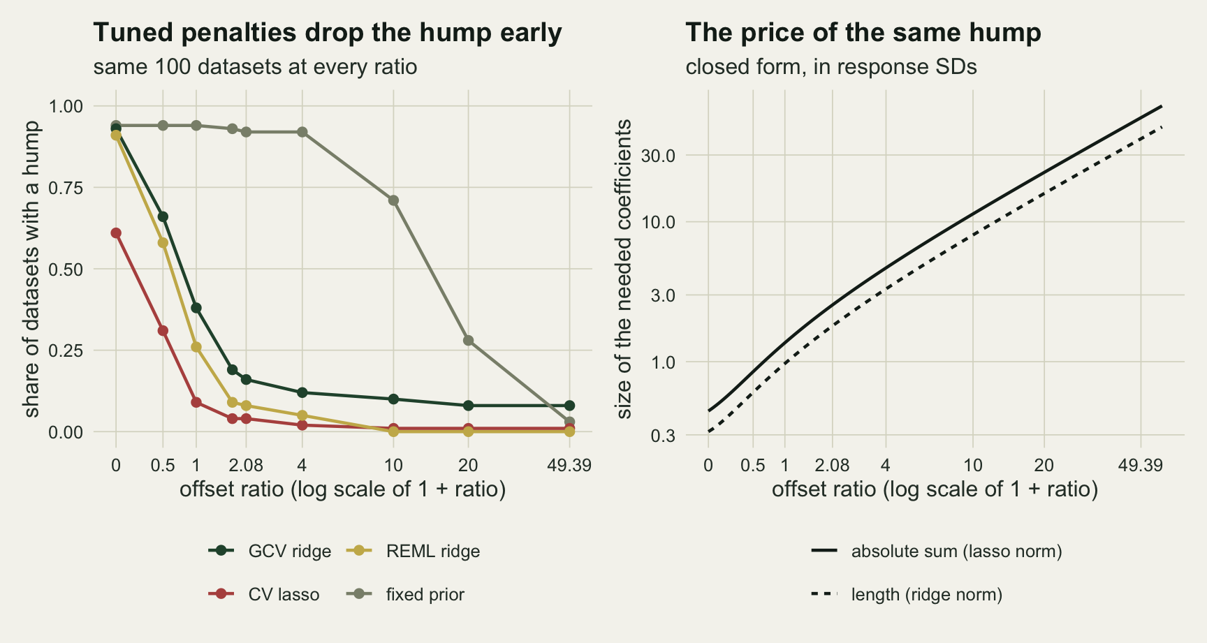
A lost hump, not a moved optimum
anch <- main_res[main_res$n == 60 & main_res$r2_t == 0.1, ]
opt_stat <- function(m, cn) {
  v <- anch$opt_err[anch$method == m & anch$coding == cn & anch$hump == 1]
  c(count = length(v), med_abs = median(abs(v)))
}
rmse_at <- function(m, cn) mean(anch$rmse[anch$method == m & anch$coding == cn])
mono_share <- function(m, cn) {
  a <- anch[anch$method == m & anch$coding == cn & anch$hump == 0, ]
  mean(a$b_u2 >= 0 | abs(a$b_u2) < 1e-12)
}
When a penalised fit on Celsius does find a hump, the optimum it reports is somewhat worse than the least squares one but on the same scale, not off by the width of the gradient. GCV ridge found 16 humps out of 100 on Celsius, with a median absolute optimum error of 1.69 C, against 93 humps and 1.03 C centred. The lasso found 4 on Celsius (median error 1.41 C) and 61 centred (1.25 C). Least squares, for comparison, is at 1.13 C on 94 humps. These errors are conditional on a hump being found, and on Celsius they rest on a handful of fits, so the counts belong next to them. A median error 0.56 C larger than that of least squares (on 16 fits against 94) is a worse estimate; for GCV ridge on Celsius the larger loss is the 84 datasets out of 100 in which no optimum is reported at all.
The failure is the other kind: the curve stops being a hump. The curve error measures that, and it moves in the direction of the hump shares. Averaged over the 100 anchor datasets it is 0.45 for least squares in any coding, 0.48 for GCV ridge centred against 0.72 on Celsius, and 0.55 for the lasso centred against 0.74. The figure below shows the failure on one dataset, chosen by a stated rule: the first anchor dataset in which centred GCV ridge finds the hump and Celsius GCV ridge does not.
pick <- which(sapply(seq_len(n_ds), function(d)
  anch$hump[anch$ds == d & anch$method == "gcv" & anch$coding == "centred"] == 1 &&
  anch$hump[anch$ds == d & anch$method == "gcv" & anch$coding == "celsius"] == 0))[1]
ex <- anchor_sites[[pick]]; ex_grid <- seq(min(ex$temp), max(ex$temp), length.out = 200)
ex_curves <- do.call(rbind, lapply(c("centred", "celsius"), function(cn) {
  X <- coded_design(ex, codings[[cn]])
  fits <- list(ols = coef(lm(ex$y ~ X)), gcv = fit_ridge_gcv(X, ex$y)$coef,
               lasso = fit_lasso_cv(X, ex$y, ex$folds)$coef)
  do.call(rbind, lapply(names(fits), function(m) {
    v <- quad_curve(fits[[m]], ex, codings[[cn]])(ex_grid)
    data.frame(temp = ex_grid, value = v - mean(v), fit = meth_lab[[m]],
               coding = paste("temperature", coding_lab[[cn]]))
  }))
}))
ex_truth <- -(ex_grid - t_opt)^2
ex_truth <- sqrt(ex$r2_t) * (ex_truth - mean(ex_truth)) / sd(-(ex$temp - t_opt)^2)
truth_df <- data.frame(temp = rep(ex_grid, 2), value = rep(ex_truth, 2),
                       coding = rep(paste("temperature", coding_lab[c("centred", "celsius")]), each = 200))
ex_curves$coding <- factor(ex_curves$coding, levels = unique(ex_curves$coding))
truth_df$coding <- factor(truth_df$coding, levels = levels(ex_curves$coding))
ex_curves$fit <- factor(ex_curves$fit, levels = meth_lab[1:3])
ggplot(ex_curves, aes(temp, value, colour = fit)) +
  geom_line(data = truth_df, aes(temp, value), inherit.aes = FALSE,
            colour = te_body, linetype = "dashed", linewidth = 0.7) +
  geom_line(linewidth = 0.9) +
  facet_wrap(~coding) +
  scale_colour_manual(values = meth_col, name = NULL) +
  labs(x = "temperature (C)", y = "fitted thermal effect (response SDs)",
       title = "Same reaches, same penalty, different zero",
       subtitle = "least squares is identical in both panels") +
  theme_datasheet() + theme(legend.position = "bottom")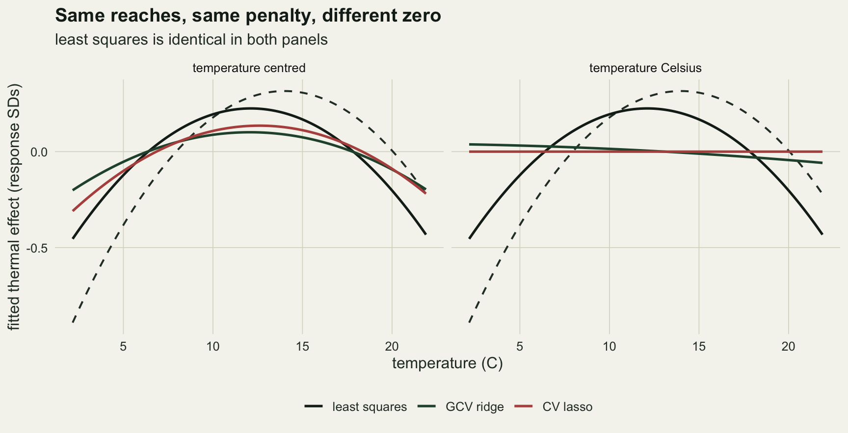
REML ridge, checked twice
REML ridge is the one penalty that does not recover as the signal strengthens, and a collapse that complete is worth a second implementation before it is printed. The model behind it is y = a + Zb + e with the slopes b drawn from a normal distribution with one shared variance tau2 and the errors from one with variance s2. Its restricted likelihood can be written out through the singular values of the standardised design; with s2 profiled out it is a function of the penalty s2 / tau2 alone, which is searched on a grid of log penalties from -10 to 25 and refined with optimize. That penalty should equal the smoothing parameter mgcv reports. The agreement criterion was set before comparing: the two penalties within 1 per cent of each other in at least 95 per cent of fits. A first version searched both log variances at once with BFGS in optim, and it stopped early on flat stretches of the likelihood in some fits; the profiled search replaced it.
reml_by_hand <- function(X, y, log_lim = c(-10, 25)) {
  st <- standardise_cols(X); Z <- st$Z; n <- nrow(Z); yc <- y - mean(y)
  sv <- svd(Z); d2 <- sv$d^2
  w2 <- as.numeric(crossprod(sv$u, yc))^2; r2 <- sum(yc^2) - sum(w2)
  neg_rl <- function(ll) {                  # lambda = s2 / tau2, s2 profiled out
    v <- 1 + d2 / exp(ll); s2 <- (sum(w2 / v) + r2) / (n - 1)
    0.5 * ((n - 1) * log(s2) + sum(log(v)))
  }
  lg <- seq(log_lim[1], log_lim[2], length.out = 141)
  k <- which.min(sapply(lg, neg_rl)); boundary <- k == length(lg)
  ll <- if (boundary) log_lim[2] else
    optimize(neg_rl, lg[c(max(k - 1, 1), k + 1)], tol = 1e-10)$minimum
  rp <- ridge_svd(Z, yc, exp(ll), sv)
  list(coef = to_raw_scale(rp$B[, 1], st, mean(y))[, 1], lambda = exp(ll), boundary = boundary)
}
reml_rows <- list()
for (d in seq_len(n_ds)) for (cn in names(codings)) {
  X <- coded_design(anchor_sites[[d]], codings[[cn]]); h <- reml_by_hand(X, anchor_sites[[d]]$y)
  m <- fit_ridge_reml(X, anchor_sites[[d]]$y); sc <- standardise_cols(X)$scl
  reml_rows[[length(reml_rows) + 1]] <- data.frame(coding = cn, rel = h$lambda / m$lambda - 1,
    boundary = h$boundary, lam_mgcv = m$lambda, slope_mgcv = max(abs(m$coef[-1] * sc)),
    hump = score_curve(quad_curve(h$coef, anchor_sites[[d]], codings[[cn]]), anchor_sites[[d]])[["hump"]])
}
reml_chk <- do.call(rbind, reml_rows)
inner <- !reml_chk$boundary
reml_agree <- mean(abs(reml_chk$rel[inner]) < 0.01); reml_maxrel <- max(abs(reml_chk$rel[inner]))
n_bound <- sum(reml_chk$boundary); bound_lam <- min(reml_chk$lam_mgcv[reml_chk$boundary])
bound_slope <- max(reml_chk$slope_mgcv[reml_chk$boundary])
hand_share <- tapply(reml_chk$hump, reml_chk$coding, mean)
reml_strong <- cell_tab$hump[cell_tab$method == "reml" & cell_tab$n == 150 & cell_tab$r2_t == 0.3]
names(reml_strong) <- cell_tab$coding[cell_tab$method == "reml" & cell_tab$n == 150 & cell_tab$r2_t == 0.3]
nuis_std <- sqrt(share_nuis) * w_nuis / sqrt(sum(w_nuis^2))   # true standardised nuisance slopes
hump_vs_nuis <- max(abs(price_tab[c("b_lin", "b_sq"), "celsius"])) / max(abs(nuis_std))
Of the 400 fits (all four codings of the 100 anchor datasets), 31 have their restricted likelihood maximum on the boundary where the shared variance is zero and the penalty is infinite. A ratio of two infinite penalties is not defined, so the 1 per cent criterion cannot apply to them; there the hand-coded fit sets every slope to zero, and mgcv stops at a penalty of at least 505120 with no standardised slope larger than \(2.9 \times 10^{-5}\), which the flatness rule scores as no hump. On the other 369 fits the two penalties agree within 1 per cent in 100 per cent, with a largest relative difference of \(5.9 \times 10^{-3}\), so the criterion is met. The hand-coded fit finds the hump in 91 per cent of datasets centred and 8 per cent on Celsius; mgcv gives 91 and 8 per cent. With a strong signal and 150 reaches, where the other penalties have recovered, REML ridge still finds the hump in 100 per cent of datasets centred and 6 per cent on Celsius. The median REML penalty at the anchor is 65 centred and 94 on Celsius, which against a smallest eigenvalue of 1.34 leaves the hump direction a fraction 0.014 of its size.
The reason is in what REML is asked to estimate. One variance is shared by eighteen slopes, thirteen of them exactly zero in truth, so the estimated variance is small. Centred, the hump needs two standardised coefficients of 0.19 and -0.25, the same size as the three real nuisance slopes (0.29, -0.22 and 0.14), and they fit under that variance. On Celsius it needs +1.36 and -1.19, the larger of them 4.7 times the largest nuisance slope, which a small shared variance treats as implausible. This is not a verdict on REML. In the tensor product post it is the REML score that recovers the right rescaling of a covariate. What fails here is the prior it was given: an exchangeable variance for coefficients that the coding has made very unequal.
A fixed prior is not an estimated one
A fixed, weakly informative prior is the Bayesian user’s default, and it is not the same object as the REML variance, so it is kept apart in every number. The version used here puts a normal prior with standard deviation 2.5 times the standard deviation of the response on every standardised slope, which is the Gaussian-model default of rstanarm (a normal prior with scale 2.5 sd(y) on standardised inputs). That default carries over the fixed-scale idea Gelman and colleagues 2008 proposed for logistic regression, where they put a Cauchy prior with scale 2.5 on inputs rescaled to a standard deviation of 0.5. The fit takes the joint posterior mode with the error variance.
fx_share <- sapply(names(codings), function(cn) share_of("fixed", cn))
fx_lam <- lam_med("fixed", "celsius")
fx_rmse <- sapply(names(codings), function(cn) rmse_at("fixed", cn))
On the anchor datasets the fixed prior finds the hump in 94 per cent centred, 92 per cent on Celsius, 92 per cent at a ratio of 4 and 3 per cent in kelvin. Its penalty is not tuned; at the median it is 0.08, far below what GCV or REML chose, and small against the Celsius eigenvalue of 1.34. That is why it behaves almost like least squares at Celsius. In kelvin the smallest eigenvalue is \(2.5 \times 10^{-3}\), far below even this penalty, and the hump is gone. A fixed prior has the same origin problem as the tuned penalties; it simply has its threshold much further out, because it shrinks so little. The two extra ratios of the offset figure place it: the fixed prior finds the hump in 71 per cent of the anchor datasets at a ratio of 10 and 28 per cent at 20. Its curve error is 0.45 centred and 0.72 in kelvin.
Repairs that remove the origin
Three repairs take the origin out of the problem rather than hoping the penalty is weak. Centring before squaring is the first, and it is what the centred coding already is. Orthogonal polynomials, poly(temp, 2), are the second: they are centred and orthogonalised inside the call, so the same columns come out whatever the origin of the input. The third is a smooth, s(temp) in mgcv, with the nuisance columns under the same ridge penalty as before; its wiggliness penalty acts on the second derivative, which a shift of origin does not change.
fit_repair <- function(s, ratio, method) {
  shift <- ratio * sd(s$temp) - mean(s$temp); u <- s$temp + shift
  if (method == "smooth") {
    zn <- standardise_cols(cbind(s$nuis, s$nuis2))$Z
    g <- gam(s$y ~ s(u, k = 10) + zn, paraPen = list(zn = list(diag(ncol(zn)))), method = "REML")
    cfn <- function(tt) as.numeric(predict(g, newdata = list(u = tt + shift,
             zn = matrix(0, length(tt), ncol(zn))), type = "terms")[, "s(u)"])
    return(score_curve(cfn, s))
  }
  pp <- poly(u, 2); Xp <- cbind(pp, s$nuis, s$nuis2)
  f <- if (method == "poly_gcv") fit_ridge_gcv(Xp, s$y) else fit_lasso_cv(Xp, s$y, s$folds)
  b <- unname(f$coef)
  score_curve(function(tt) as.numeric(predict(pp, tt + shift) %*% b[2:3]), s)
}
rep_methods <- c("poly_gcv", "poly_lasso", "smooth")
rep_rows <- list()
for (d in seq_len(n_ds)) for (cn in c("centred", "kelvin")) for (m in rep_methods)
  rep_rows[[length(rep_rows) + 1]] <- c(ds = d, kelvin = cn == "kelvin", method = match(m, rep_methods),
                                        fit_repair(anchor_sites[[d]], codings[[cn]], m))
rep_res <- as.data.frame(do.call(rbind, rep_rows)); rep_res$method <- rep_methods[rep_res$method]
rep_gap <- max(abs(rep_res$rmse[rep_res$kelvin == 1] - rep_res$rmse[rep_res$kelvin == 0]))
rep_share <- tapply(rep_res$hump[rep_res$kelvin == 0], rep_res$method[rep_res$kelvin == 0], mean)
rep_rmse <- tapply(rep_res$rmse[rep_res$kelvin == 0], rep_res$method[rep_res$kelvin == 0], mean)
la_c <- anch[anch$method == "lasso" & anch$coding == "centred", ]
viol_c <- mean(la_c$b_u == 0 & la_c$b_u2 != 0)
is_viol <- la_c$b_u == 0 & la_c$b_u2 != 0 & la_c$hump == 1
viol_opt <- median(la_c$opt_err[is_viol])
t_means <- sapply(anchor_sites, function(s) mean(s$temp))
viol_pin <- max(abs(la_c$opt_err[is_viol] - (t_means[la_c$ds[is_viol]] - t_opt)))
t_mean_avg <- mean(t_means); t_mean_viol <- mean(t_means[la_c$ds[is_viol]])
tuned <- anch[anch$method %in% c("gcv", "lasso", "reml"), ]
tuned_best <- min(c(tapply(tuned$rmse, paste(tuned$method, tuned$coding), mean), rep_rmse))
fixed_best <- min(sapply(names(codings), function(cn) rmse_at("fixed", cn)))
Fitted in the centred and the kelvin coding, the two polynomial fits and the smooth give curve errors that differ by at most \(3.1 \times 10^{-14}\), so each repair is one answer whatever the origin. GCV ridge on poly() columns finds the hump in 95 per cent of the anchor datasets and the lasso on them returns a hump in 61 per cent, close to the centred shares of 93 and 61 per cent. The smooth finds a hump in 76 per cent with a curve error of 0.47: its own penalty shrinks towards a straight line, which is the right null for a smooth and a separate question from the origin.
Centring does not make the lasso hierarchical. In 27 per cent of the centred lasso fits the squared term is kept and the linear one dropped, the violation Peixoto’s rule forbids. In the centred coding that model is a hump with its vertex pinned at the mean temperature of the sample: the reported optimum equals the sample mean to within 0.005 C in every such fit, and the median optimum error is -1.41 C. That is smaller than the gap between the true optimum and the average sample mean of 12.1 C, because the lasso drops the linear term more readily in samples whose mean happens to lie nearer the optimum (their average is 12.7 C). The dropped linear term puts the optimum wherever zero was put. A lasso on poly() columns that keeps the quadratic column without the linear one pins the vertex in the same way, at a point fixed by the sample. Centring buys a hump but not a free vertex; the hierarchical lasso of Bien, Taylor and Tibshirani 2013 is the fit that removes both problems at once, and it is not coded here.
rep_lab <- data.frame(
  label = c("least squares, any coding", "GCV ridge, Celsius", "GCV ridge, centred", "GCV ridge, poly()",
            "CV lasso, Celsius", "CV lasso, centred", "CV lasso, poly()", "REML ridge, Celsius",
            "REML ridge, centred", "fixed prior, kelvin", "fixed prior, Celsius", "s(temp) smooth"),
  hump = c(share_of("ols", "celsius"), h_gcv_k, h_gcv_c, rep_share[["poly_gcv"]], h_lasso_k, h_lasso_c,
           rep_share[["poly_lasso"]], share_of("reml", "celsius"), share_of("reml", "centred"),
           fx_share[["kelvin"]], fx_share[["celsius"]], rep_share[["smooth"]]),
  rmse = c(rmse_at("ols", "celsius"), rmse_at("gcv", "celsius"), rmse_at("gcv", "centred"), rep_rmse[["poly_gcv"]],
           rmse_at("lasso", "celsius"), rmse_at("lasso", "centred"), rep_rmse[["poly_lasso"]],
           rmse_at("reml", "celsius"), rmse_at("reml", "centred"), fx_rmse[["kelvin"]], fx_rmse[["celsius"]],
           rep_rmse[["smooth"]]),
  kind = c("control", "uncentred coding", "origin removed", "origin removed", "uncentred coding", "origin removed",
           "origin removed", "uncentred coding", "origin removed", "uncentred coding", "uncentred coding", "origin removed"))
rep_lab$label <- factor(rep_lab$label, levels = rev(rep_lab$label))
kind_col <- c("control" = te_ink, "uncentred coding" = te_rust, "origin removed" = te_forest)
p_h <- ggplot(rep_lab, aes(hump, label, colour = kind)) +
  geom_segment(aes(x = 0, xend = hump, yend = label), linewidth = 0.5) + geom_point(size = 2.4) +
  scale_colour_manual(values = kind_col, name = NULL) + scale_x_continuous(limits = c(0, 1)) +
  labs(x = "share with a hump", y = NULL, title = "Hump found") +
  theme_datasheet() + theme(legend.position = "bottom")
p_r <- ggplot(rep_lab, aes(rmse, label, colour = kind)) +
  geom_point(size = 2.4) +
  scale_colour_manual(values = kind_col, name = NULL) +
  labs(x = "curve error (SDs of the true curve)", y = NULL, title = "Curve error") +
  theme_datasheet() + theme(legend.position = "none", axis.text.y = element_blank())
p_h + p_r + plot_annotation(theme = theme_datasheet())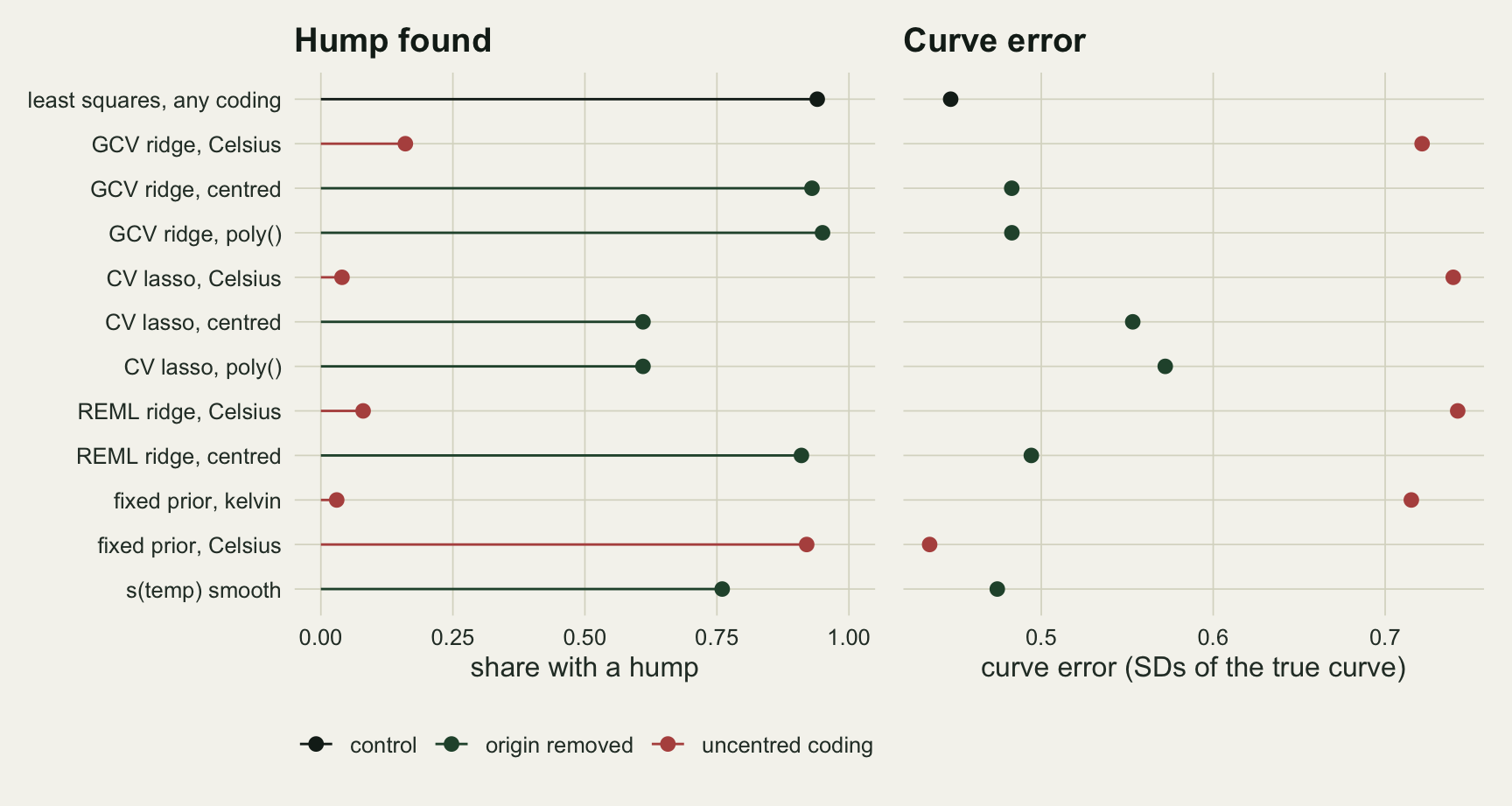
What to report
Say how a squared covariate was coded before it went into a penalised fit: the origin, not only the unit. “Temperature and its square, standardised” does not say where zero was, and under a penalty that sentence does not identify the model.
Centre before squaring, or use poly(), and say which. Standardising afterwards is fine, and it is still needed for the unit, but it is not a substitute; the same holds for products of covariates in an interaction.
If a published penalised fit reports a monotone response to a covariate that was squared in an uncentred coding, the monotone shape is not evidence against an optimum. Refit centred before reading anything into it.
For a lasso, report whether the squared term was kept without its linear term. In a centred coding that model puts the optimum at the sample mean by construction, and that optimum is a property of the sample, not of the species.
When the penalty is estimated as a shared variance, as in REML ridge or a hierarchical prior, check whether the coding has made one or two coefficients much larger than the rest. An exchangeable prior assumes they are not.
Honest limits
The true response is exactly quadratic, so least squares on the quadratic is the correctly specified model. At the anchor its curve error of 0.447 is lower than that of every tuned fit and every repair, the best of which reaches 0.474; only the fixed weak prior, which barely shrinks, edges below it at 0.429. The penalties may earn their keep in designs with many more useless columns than here, or with weaker signals; neither was swept. The claim this post supports is that the penalised answer depends on the origin, not that a penalty was the right tool for this dataset.
Only Gaussian responses were simulated. A presence-absence or count version with a penalised logistic or Poisson fit should suffer the same way, because the penalty still prices standardised coefficients of the same collinear pair, but that was not run, and MaxEnt’s own loss was not run either. The MaxEnt paragraph rests on the arithmetic of its rescaling and of its per-feature penalty, not on a MaxEnt fit.
Temperature is uniform on the sampled range. For a skewed covariate, centring still removes the origin, but the centred variable stays correlated with its square, so the penalty still prices the hump as a pair of correlated coefficients; poly() removes that correlation as well. That is a different parametrisation, not a more complete repair of the origin, and it was not simulated here. The closed forms for the correlation and the coefficient sizes are for the uniform only.
The GCV penalty grid runs from \(10^{-4}\) to \(10^{4}\), and the lasso grid spans three orders of magnitude below the largest penalty. Across all cells and codings GCV chose the top of its grid in 1.8 per cent of fits and the bottom in 5.4 per cent. At the top every slope is already shrunk almost to nothing (7 per cent of those fits find a hump), and a larger cap could only shrink further; at the bottom the fit is already least squares in all but name. The lasso chose the smallest penalty on its grid in 11.6 per cent of fits, and 100 per cent of those already find the hump, so a lower floor could not add any. The grids are not what drives the result. The five folds are one random draw per dataset, shared across codings, and the effect of redrawing them was not measured.
Each design cell is 100 datasets and one seed, fixed before any rate was examined. The Monte Carlo standard error of a share is at most 0.050, so differences of a few points between codings of the tuned penalties at a ratio of 4 and beyond are not worth reading.
References
Peixoto JL 1987 The American Statistician 41(4):311-313 (10.1080/00031305.1987.10475506)
Bien J, Taylor J, Tibshirani R 2013 Annals of Statistics 41(3):1111-1141 (10.1214/13-AOS1096)
Hoerl AE, Kennard RW 1970 Technometrics 12(1):55-67 (10.1080/00401706.1970.10488634)
Gelman A, Jakulin A, Pittau MG, Su YS 2008 Annals of Applied Statistics 2(4):1360-1383 (10.1214/08-AOAS191)