library(ggplot2)
library(patchwork)

te_paper  <- "#f5f4ee"
te_ink    <- "#16241d"
te_body   <- "#2c3a31"
te_forest <- "#275139"
te_rust   <- "#b5534e"
te_gold   <- "#c9b458"
te_line   <- "#dad9ca"

theme_datasheet <- function() {
  theme_minimal(base_size = 12) +
    theme(plot.background  = element_rect(fill = te_paper, colour = NA),
          panel.background = element_rect(fill = te_paper, colour = NA),
          panel.grid.major = element_line(colour = te_line, linewidth = 0.3),
          panel.grid.minor = element_blank(),
          text             = element_text(colour = te_body),
          plot.title       = element_text(colour = te_ink, face = "bold"),
          plot.subtitle    = element_text(colour = te_body),
          axis.text        = element_text(colour = te_body))
}Parameter scale decides what optim() finds
R
numerical methods
likelihood
population dynamics
reproducibility
ecology tutorial
One Ricker fit, two spellings: optim BFGS in (r, K) stops far below the exact carrying capacity, and raising maxit makes it report success. Why, and the fix.
Thirty summers of counts from a seabird colony, a few hundred pairs at the start and several thousand by the end. The model is the Ricker (Ricker 1954), the one every population course teaches: next year’s log growth is a maximum rate r, pulled down in proportion to how close this year’s count is to a carrying capacity K, plus process noise. The analyst writes the negative log-likelihood in r, K and the log of the noise standard deviation, picks a start, and calls optim(start, nll, method = "BFGS"), which is how the function is called in the help page and in a large share of the posts on this site. The call returns a carrying capacity more than a third too small. A third of the time it also returns convergence code 0; the rest of the time it returns code 1, and raising maxit turns many of those into a 0, about half of them with K still more than a tenth out.
Nothing about this is new. Gradient methods are not scale invariant: a parameter whose natural size is thousands, sitting next to parameters whose natural size is about one, gets moved by the search as if it were the same size as the others. Nash and Varadhan 2011 discuss scaling diagnostics for optim() and its relatives, and the remedy, the parscale element of the control list, is documented accurately on the help page. What this post measures is how large the damage is on an ordinary ecological fit, why the one warning a reader gets disappears under the obvious fix, and which of the other fitters in base R share the problem. The mechanism is traced step by step, down to one line of R’s C source, because the two tempting explanations both turn out to be wrong.
The nearest posts on the site are about fitting too, and the difference matters. Starting values and identifiability in nls reparameterises a decay curve by shifting its time origin, which removes a correlation between parameters while “the rate estimate is unchanged”; there the new spelling makes the fit cleaner and moves no answer. Checking a mixture model asks which of several optima a run found. Here there is one optimum, every fitter starts at the same point, and two algebraically identical spellings of the same model disagree about the carrying capacity by more than a third. The theta-logistic model in R calls BFGS with maxit = 2000, the reflex this post puts a number on, but fits K on the log scale, log(max(N) * 1.05), which is the repair applied without comment. When integrate() in R returns zero and says OK is the sibling case: an undeclared default inside a base R function that fails while reporting success.
There is also a reason this particular fit should never have gone wrong, and it is part of the lesson. Written with b = r / K instead of K, the Ricker on the log scale is a straight line in this year’s count, so lm() returns the exact maximum likelihood estimate with no search at all. That exact answer is the benchmark throughout. Nothing below is compared with the true K or with the best of the fitters; every error is measured against the exact maximum of the same likelihood, on the same series.
One model, two spellings
The generating model is the stochastic Ricker on the log scale, with a maximum growth rate of 0.45, a carrying capacity of 5000, a process standard deviation of 0.25 and a first count of 800. Every series is thirty years long. The likelihood is the normal density of the one-step log growth, with the log of sigma as the third parameter so that no parameter has a bound.
r_true   <- 0.45     # maximum per capita log growth
K_true   <- 5000     # carrying capacity
sd_proc  <- 0.25     # process noise on the log scale
N_first  <- 800      # first count
n_yr     <- 30       # years per series
start_far <- c(0.30, 3000, log(0.3))   # r, K, log sigma: fixed before any fit was run
box_lo <- c(-2, 10, -5); box_hi <- c(5, 1e6, 5)

sim_ricker <- function() {
  N <- numeric(n_yr); N[1] <- N_first
  for (i in 2:n_yr)
    N[i] <- N[i - 1] * exp(r_true * (1 - N[i - 1] / K_true) + rnorm(1, 0, sd_proc))
  N
}

make_fit <- function(N) {
  y <- diff(log(N)); x <- N[-length(N)]
  cf <- coef(lm(y ~ x))
  r_ex <- unname(cf[1]); b_ex <- -unname(cf[2])
  s_ex <- sqrt(mean((y - (r_ex - b_ex * x))^2))      # the MLE of sigma divides by n
  nll_K <- function(th) {
    if (th[2] <= 1) return(1e12)
    -sum(dnorm(y - th[1] * (1 - x / th[2]), 0, exp(th[3]), log = TRUE))
  }
  nll_b <- function(th) -sum(dnorm(y - (th[1] - th[2] * x), 0, exp(th[3]), log = TRUE))
  list(y = y, x = x, r_ex = r_ex, b_ex = b_ex, K_ex = r_ex / b_ex, ls_ex = log(s_ex),
       nll_K = nll_K, nll_b = nll_b, nll_ex = nll_b(c(r_ex, b_ex, log(s_ex))))
}
The two negative log-likelihoods are the same function of the data. One takes (r, K, log sigma); the other takes (r, b, log sigma) with b = r / K. Before anything is fitted it is worth checking that they agree and that the lm() point really is the maximum.
set.seed(77)
N_one  <- sim_ricker()
fm_one <- make_fit(N_one)
th_K <- c(fm_one$r_ex, fm_one$K_ex, fm_one$ls_ex)
th_b <- c(fm_one$r_ex, fm_one$b_ex, fm_one$ls_ex)
same_gap <- abs(fm_one$nll_K(th_K) - fm_one$nll_b(th_b))
polish   <- nlminb(th_K, fm_one$nll_K)
polish_gain <- fm_one$nll_ex - polish$objective
polish_move <- abs(polish$par[2] - fm_one$K_ex) / fm_one$K_ex
On one simulated series the two spellings differ in the negative log-likelihood by less than one in a billion at the lm() point. Handing that point to nlminb() as a start changes the negative log-likelihood by less than one in a billion and K by a fraction of exactly zero: the linear regression is the maximum, and the search has nowhere better to go. The exact carrying capacity for this series is 5509 and the exact r is 0.560.
Ten calls from one start
Ten ways of maximising the same likelihood, all from the same start of r = 0.30, K = 3000 and sigma = 0.3, expressed identically in both spellings. The start is a plausible guess by someone who knows the colony is in the low thousands; it is fixed in the code above, and a second, more careful start is tried later. Four of the calls are BFGS in (r, K): the default call, the same call with maxit = 5000, the same call with the finite-difference step ndeps shrunk to \(10^{-6}\), and the same call with parscale = c(1, 3000, 1), which tells optim() that K is about three thousand times larger than the other two parameters. The fifth is BFGS in (r, b). Then come Nelder-Mead (Nelder and Mead 1965), which uses no gradient, and L-BFGS-B and nlminb(), each run with and without box bounds, since the bounded versions are how most people call them.
fit_lab <- c(def  = "BFGS, default",       maxit = "BFGS, maxit = 5000",
             nd6  = "BFGS, ndeps = 1e-6",  pars  = "BFGS, parscale",
             rb   = "BFGS in (r, b)",      nm    = "Nelder-Mead",
             lb   = "L-BFGS-B, box",       lbn   = "L-BFGS-B, no box",
             nlb  = "nlminb, box",         nlbn  = "nlminb, no box")

one_row <- function(o, form = "K")
  c(K = if (form == "K") o$par[2] else o$par[1] / o$par[2],
    nll = o$value, code = o$convergence)
nlm_row <- function(o) c(K = o$par[2], nll = o$objective, code = o$convergence)

run_fitters <- function(fm, st, which = names(fit_lab)) {
  sb <- c(st[1], st[1] / st[2], st[3]); ps <- c(1, st[2], 1)
  calls <- list(
    def   = function() one_row(optim(st, fm$nll_K, method = "BFGS")),
    maxit = function() one_row(optim(st, fm$nll_K, method = "BFGS",
                                     control = list(maxit = 5000))),
    nd6   = function() one_row(optim(st, fm$nll_K, method = "BFGS",
                                     control = list(ndeps = rep(1e-6, 3)))),
    pars  = function() one_row(optim(st, fm$nll_K, method = "BFGS",
                                     control = list(parscale = ps))),
    rb    = function() one_row(optim(sb, fm$nll_b, method = "BFGS"), "b"),
    nm    = function() one_row(optim(st, fm$nll_K, method = "Nelder-Mead",
                                     control = list(maxit = 2000, reltol = 1e-11))),
    lb    = function() one_row(optim(st, fm$nll_K, method = "L-BFGS-B",
                                     lower = box_lo, upper = box_hi)),
    lbn   = function() one_row(optim(st, fm$nll_K, method = "L-BFGS-B")),
    nlb   = function() nlm_row(nlminb(st, fm$nll_K, lower = box_lo, upper = box_hi)),
    nlbn  = function() nlm_row(nlminb(st, fm$nll_K)))
  vapply(calls[which], function(f) f(), numeric(3))
}

n_blk <- 5; n_ser <- 100          # fixed before any rate was inspected
series <- unlist(lapply(seq_len(n_blk), function(bl) {
  set.seed(1000 + bl)
  lapply(seq_len(n_ser), function(i) sim_ricker())
}), recursive = FALSE)
blk <- rep(seq_len(n_blk), each = n_ser)
fms <- lapply(series, make_fit)
K_ex  <- vapply(fms, function(f) f$K_ex, 0)
nll_ex <- vapply(fms, function(f) f$nll_ex, 0)
t_main <- system.time(
  res_far <- vapply(fms, run_fitters, matrix(0, 3, length(fit_lab)), st = start_far)
)[["user.self"]]
dimnames(res_far)[[2]] <- names(fit_lab)
rel_err <- function(res, f) (res["K", f, ] - K_ex) / K_ex
summ <- function(res, f, st_K) {
re <- rel_err(res, f)
data.frame(fitter = f,
block = seq_len(n_blk),
med_rel = tapply(abs(re), blk, median),
off10 = tapply(abs(re) > 0.10, blk, mean),
code0 = tapply(res["code", f, ] == 0, blk, mean),
deficit = tapply(res["nll", f, ] - nll_ex, blk, median),
below = tapply(re < 0, blk, mean))
}
tab_far <- do.call(rbind, lapply(names(fit_lab), function(f) summ(res_far, f)))
rng <- function(f, col, d = 3, tab = tab_far, as_pct = FALSE) {
v <- tab[tab$fitter == f, col]
if (as_pct) v <- 100 * v
paste(sprintf(paste0("%.", d, "f"), range(v)), collapse = " to ")
}
pool <- function(f, fun, res = res_far) fun(res, f)
share_code0 <- function(res, f) mean(res["code", f, ] == 0)
share_off <- function(res, f) mean(abs(rel_err(res, f)) > 0.10)
med_abs <- function(res, f) median(abs(rel_err(res, f)))
n_all <- n_blk * n_ser
mcse_share <- function(p) sqrt(p * (1 - p) / n_all)
exact_set <- c("pars", "rb", "nm", "nlb", "nlbn")
worst_exact <- max(vapply(exact_set, function(f) max(abs(rel_err(res_far, f))), 0))
chi_half <- qchisq(0.95, 1) / 2 # profile-likelihood cut-off for a 95 per cent intervalThe default BFGS call in (r, K) lands a median 35.7 to 39.9 per cent away from the exact carrying capacity, per block of 100 series, and it errs downwards, towards the start: in 99.4 per cent of all 500 series the fitted K is below the exact one. The share more than ten per cent off is 0.97 to 0.99 per block, and the median shortfall in log-likelihood against the exact maximum is 4.62 to 4.99 units, which is not a rounding difference: a 95 per cent profile-likelihood interval for one parameter reaches only 1.92 units below the maximum. The fit reports convergence code 0 in 0.27 to 0.39 of the series in a block.
Five of the ten calls find the exact maximum every time, to within the tolerance of the search. BFGS with parscale, BFGS in (r, b), Nelder-Mead and nlminb() with and without bounds all return the lm() answer, and the largest relative error in K among them over all 500 series is 0.000082. Those five report code 0 in every series. The two L-BFGS-B calls are exact in median but not every time, and they get their own section below.
pct <- function(v) ifelse(abs(v) < 1e-9, "0%", sprintf("%+.0f%%", 100 * v))
sci_lab <- function(x) as.expression(lapply(as.character(x), function(s)   # 1e-6 as a power of ten
  if (grepl("1e-6", s, fixed = TRUE)) bquote(.(sub("1e-6", "", s, fixed = TRUE)) * 10^-6) else s))
err_long <- do.call(rbind, lapply(names(fit_lab), function(f)
  data.frame(fitter = fit_lab[[f]], err = rel_err(res_far, f),
             code0 = res_far["code", f, ] == 0)))
err_long$fitter <- factor(err_long$fitter, levels = rev(fit_lab))
err_long$status <- ifelse(err_long$code0, "reports code 0", "reports code 1")
share_df <- data.frame(fitter = factor(fit_lab, levels = rev(fit_lab)),
                       code0 = vapply(names(fit_lab), function(f) share_code0(res_far, f), 0),
                       off10 = vapply(names(fit_lab), function(f) share_off(res_far, f), 0))
set.seed(5)
p_err <- ggplot(err_long, aes(err, fitter, colour = status)) +
  geom_vline(xintercept = 0, colour = te_ink, linewidth = 0.4) +
  geom_jitter(height = 0.22, width = 0, size = 0.8, alpha = 0.55) +
  scale_colour_manual(values = c(te_forest, te_rust), name = NULL) +
  scale_x_continuous(labels = pct) + scale_y_discrete(labels = sci_lab) +
  labs(x = "fitted K relative to the exact MLE", y = NULL,
       title = "Where each call leaves K", subtitle = "one point per series, same start") +
  guides(colour = guide_legend(nrow = 2, override.aes = list(size = 2.5, alpha = 1))) +
  theme_datasheet() + theme(legend.position = "bottom")
share_long <- rbind(data.frame(fitter = share_df$fitter, share = share_df$code0,
                               what = "reports code 0"),
                    data.frame(fitter = share_df$fitter, share = share_df$off10,
                               what = "more than 10% off"))
p_share <- ggplot(share_long, aes(share, fitter, colour = what, shape = what)) +
  geom_point(size = 2.6, stroke = 1) +
  scale_colour_manual(values = c(te_rust, te_forest), name = NULL) +
  scale_shape_manual(values = c(17, 16), name = NULL) +
  scale_x_continuous(limits = c(0, 1), breaks = c(0, 0.5, 1)) + scale_y_discrete(labels = sci_lab) +
  guides(colour = guide_legend(nrow = 2), shape = guide_legend(nrow = 2)) +
  labs(x = "share of 500 series", y = NULL, title = "What the call says",
       subtitle = "and how often it is wrong") +
  theme_datasheet() + theme(legend.position = "bottom", axis.text.y = element_blank())
p_err + p_share + plot_layout(widths = c(1.6, 1)) +
  plot_annotation(theme = theme_datasheet())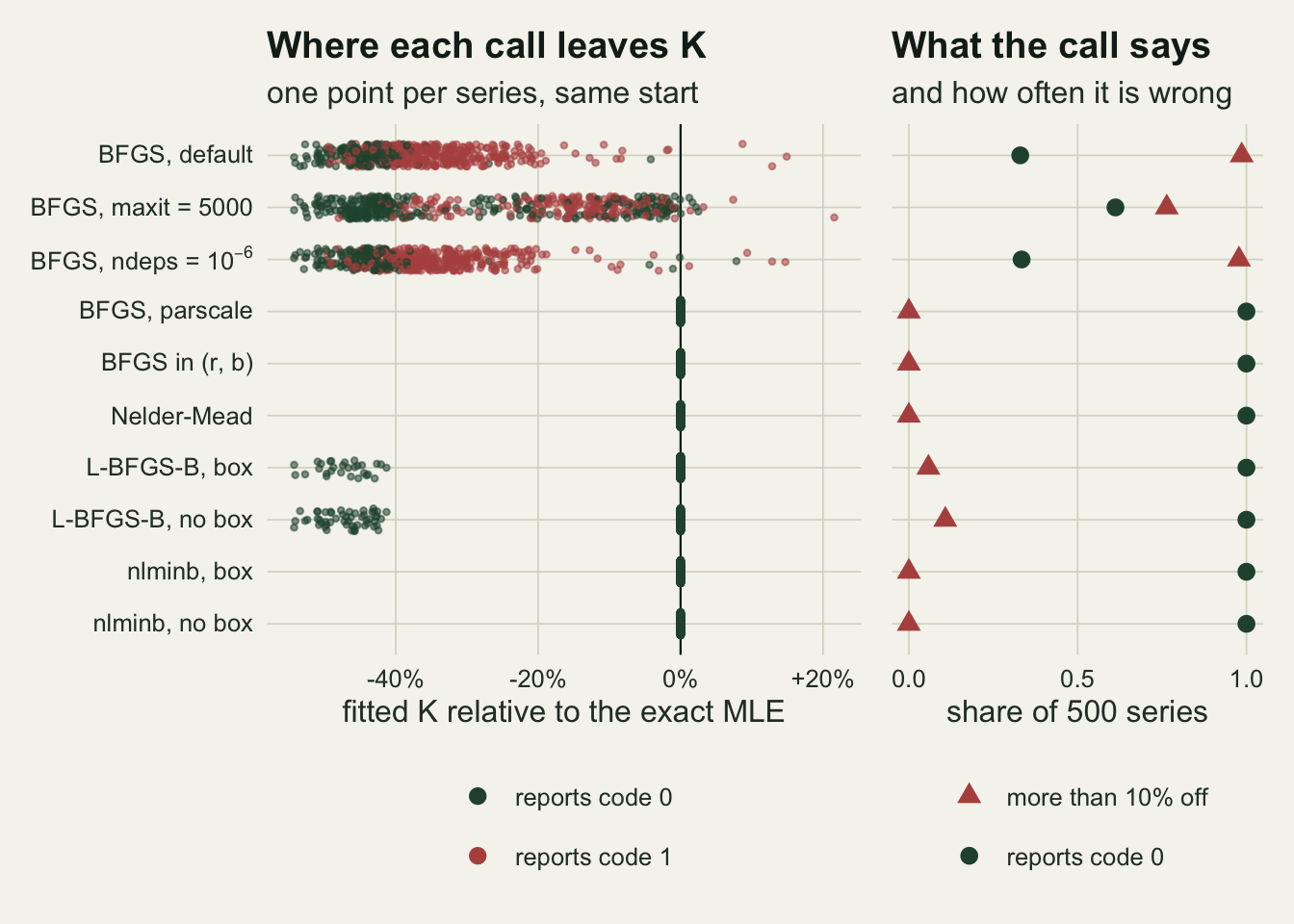
Raising maxit buys the warning away
The default BFGS call stops after 100 iterations, and when it does it returns code 1, which the help page describes as the iteration limit having been reached. A reader who checks the code sees a 1, raises maxit, reruns, and gets a 0. That is the repair everyone reaches for, and it is exactly what the site’s own fits do when they pass control = list(maxit = 2000).
code0_def <- share_code0(res_far, "def"); code0_mx <- share_code0(res_far, "maxit")
off_def <- share_off(res_far, "def");     off_mx <- share_off(res_far, "maxit")
re_mx <- rel_err(res_far, "maxit")
clean_mx <- res_far["code", "maxit", ] == 0
off_clean_mx <- mean(abs(re_mx[clean_mx]) > 0.10)
n_clean_off  <- sum(abs(re_mx[clean_mx]) > 0.10)
limit_mx <- mean(res_far["code", "maxit", ] == 1)
flip <- res_far["code", "def", ] == 1 & clean_mx
n_flip <- sum(flip); n_flip_off <- sum(abs(re_mx[flip]) > 0.10)
med_def_clean <- median(abs(rel_err(res_far, "def")[res_far["code", "def", ] == 0]))
code1_def <- res_far["code", "def", ] == 1
flip_share  <- mean(res_far["code", "maxit", code1_def] == 0)   # warnings removed
off_def_set <- abs(rel_err(res_far, "def")) > 0.10
fixed_share <- mean(abs(re_mx[off_def_set]) <= 0.10)             # errors removed
# the other lever: a tighter tolerance at the default iteration limit
res_tol <- vapply(fms, function(fm) one_row(optim(start_far, fm$nll_K, method = "BFGS",
                                           control = list(reltol = 1e-12))), numeric(3))
code0_tol <- mean(res_tol["code", ] == 0)
med_tol   <- median(abs(res_tol["K", ] - K_ex) / K_ex)
With maxit = 5000 the median relative error in K falls to 15.4 to 32.8 per cent per block, and the share of series more than ten per cent off falls to 0.67 to 0.83. Better, but still a fit that misses the carrying capacity by more than a tenth in most series. The median log-likelihood shortfall is 1.78 to 3.24 units. What changes most is the message: pooled over all 500 series, the share reporting convergence code 0 rises from 0.33 to 0.61, with a Monte Carlo standard error of at most 0.02 on each. Of the 306 series in which the raised limit reports clean convergence, 235 (77 per cent) are still more than ten per cent off, and 0.39 of all fits hit even the raised limit of 5000 iterations.
The code 0 from the default call is no safer. Among the default fits that report code 0, the median error in K is 44 per cent. The only warning the reader ever gets is a code 1, and the obvious fix removes the warning more reliably than it removes the error: of the default fits that returned code 1, 0.42 return code 0 under the raised limit, while of the default fits more than ten per cent off, only 0.23 are brought within ten per cent. Of the 141 series in which the default call said 1 and the raised limit said 0, 71 (50 per cent) are still more than ten per cent off.
The other setting a careful reader might reach for is the tolerance. Tighten reltol from its default of about \(1.5 \times 10^{-8}\) to \(10^{-12}\), leave maxit at 100, and the call reports code 0 in 0.000 of the series, with the median error in K at 37 per cent. The code 0 in the default call is the tolerance test firing, not a sign that the search got anywhere; why it fires is the subject of the next section.
mx_df <- rbind(
  data.frame(call = "BFGS, default", err = rel_err(res_far, "def"),
             deficit = res_far["nll", "def", ] - nll_ex, code = res_far["code", "def", ]),
  data.frame(call = "BFGS, maxit = 5000", err = re_mx,
             deficit = res_far["nll", "maxit", ] - nll_ex, code = res_far["code", "maxit", ]))
mx_df$status <- ifelse(mx_df$code == 0, "reports code 0", "reports code 1")
mx_df$call <- factor(mx_df$call, levels = c("BFGS, default", "BFGS, maxit = 5000"))
ggplot(mx_df, aes(err, deficit, colour = status)) +
  geom_vline(xintercept = c(-0.1, 0.1), colour = te_body, linetype = "dashed", linewidth = 0.4) +
  geom_point(size = 1.3, alpha = 0.7) +
  facet_wrap(~ call) +
  scale_colour_manual(values = c(te_forest, te_rust), name = NULL) +
  scale_x_continuous(labels = pct) +
  labs(x = "fitted K relative to the exact MLE", y = "log-likelihood below the exact maximum",
       title = "A clean convergence code on a wrong fit",
       subtitle = "dashed lines: ten per cent either side of the exact K") +
  theme_datasheet() + theme(legend.position = "bottom",
                            strip.text = element_text(colour = te_ink, face = "bold"))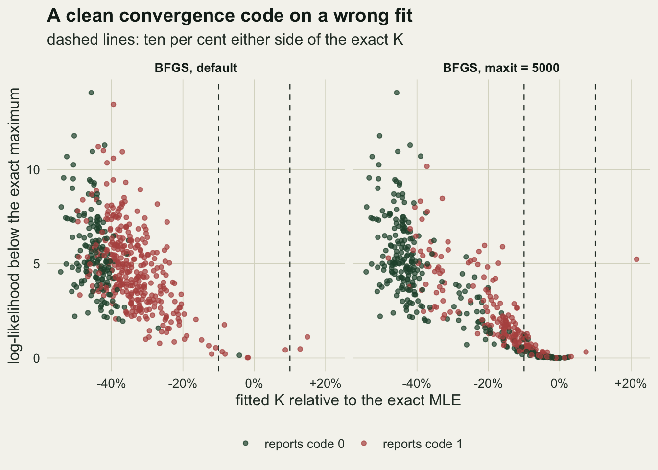
Not the gradient step: the restart
The tempting explanation is the finite-difference gradient. optim() computes the gradient by central differences with a step of ndeps = 1e-3 on each parameter, and a step of one thousandth is tiny for a parameter of size three thousand, so the gradient in K might be mostly rounding noise. That explanation is testable, and the test is already in the ten calls above: the ndeps = 1e-6 call.
nd_gap <- median(abs(res_far["K", "nd6", ] - res_far["K", "def", ]) / K_ex)Shrinking the step a thousandfold changes nothing that matters. The median relative error in K is 35.9 to 39.9 per cent per block against 35.7 to 39.9 per cent for the default, and the median difference between the two fitted values of K, per series, is 0.0000 of the exact K. The gradient is fine. What goes wrong is in how the search uses it.
The series simulated earlier shows it. Here is the gradient at the start, computed the way optim() computes it, and the path the default call takes, recorded by passing a gradient function that does the same central differences and logs every point at which it is called. The recorded call returns the same answer as the plain one, to the last digit.
num_grad <- function(f, ps = c(1, 1, 1), nd = rep(1e-3, 3)) function(th) {
  h <- nd * ps
  vapply(1:3, function(i) { e <- numeric(3); e[i] <- h[i]
    (f(th + e) - f(th - e)) / (2 * h[i]) }, 0)
}
tracked <- function(f, ctrl = list(), ps = c(1, 1, 1), nd = rep(1e-3, 3)) {
  path <- list(); g0 <- num_grad(f, ps, nd)
  gr <- function(th) { path[[length(path) + 1]] <<- th; g0(th) }
  o <- optim(start_far, f, gr, method = "BFGS", control = ctrl)
  list(o = o, path = do.call(rbind, path))
}
g_start <- num_grad(fm_one$nll_K)(start_far)
plain   <- optim(start_far, fm_one$nll_K, method = "BFGS")
tr_def  <- tracked(fm_one$nll_K)
tr_mx   <- tracked(fm_one$nll_K, list(maxit = 5000))
tr_nd   <- tracked(fm_one$nll_K, list(ndeps = rep(1e-6, 3)), nd = rep(1e-6, 3))
tr_ps   <- tracked(fm_one$nll_K, list(parscale = c(1, start_far[2], 1)),
                   ps = c(1, start_far[2], 1))
track_gap <- max(abs(plain$par - tr_def$o$par))
dist_K <- fm_one$K_ex - start_far[2]
K_moved <- tr_def$o$par[2] - start_far[2]
g_end <- num_grad(fm_one$nll_K)(plain$par)
At the start the gradient is (49.24, -0.0130, -16.32) in (r, K, log sigma). The recorded path matches the plain call exactly.
The BFGS routine inside optim() is the function vmmin in R’s source, after Nash’s variable metric code. It starts from the identity matrix, so its first direction is the raw negative gradient, and it tries a step of length 1 along that direction, shortening it by a factor of 0.2 until the function falls by enough. On that first step K can move by at most 0.0130, while the exact K for this series is 2509 pairs away. That is the second tempting explanation, the step length, and it does not hold either: a short first step is not fatal on its own. After every step the BFGS update rescales the matrix from the change in the gradient, and that is how a quasi-Newton method learns that K needs far longer steps than r. Two more lines of vmmin decide whether it gets the chance. It resets the matrix to the identity whenever more than twice as many gradients as there are parameters have been evaluated since the last reset, which here means after every seventh. And it declares convergence when a step taken straight after a reset lowers the function by less than reltol times its value.
To see which of these decides the outcome, here is vmmin transcribed into R line by line, with one switch added: restart = FALSE deletes the periodic-restart line and changes nothing else.
# BFGS as optim() runs it: a line-by-line R copy of vmmin in R's src/appl/optim.c
# restart = FALSE deletes the one periodic-restart line and changes nothing else
vmmin_r <- function(b, fn, gr, maxit = 100, reltol = sqrt(.Machine$double.eps),
                    restart = TRUE, trace = FALSE) {
  n <- length(b); f <- fn(b); Fmin <- f; g <- gr(b)
  gradcount <- 1; iter <- 1; ilast <- 1
  B <- diag(n); tt <- numeric(n); steps <- NULL
  repeat {
    if (ilast == gradcount) B <- diag(n)
    X <- b; cc <- g; gradproj <- 0
    for (i in 1:n) {
      s <- 0
      for (j in 1:i) s <- s - B[i, j] * g[j]
      if (i < n) for (j in (i + 1):n) s <- s - B[j, i] * g[j]
      tt[i] <- s; gradproj <- gradproj + s * g[i]
    }
    if (gradproj < 0) {
      steplength <- 1; accpoint <- FALSE
      repeat {
        b <- X + steplength * tt; count <- sum(10 + X == 10 + b)
        if (count < n) {
          f <- fn(b)
          accpoint <- is.finite(f) && f <= Fmin + gradproj * steplength * 1e-4
          if (!accpoint) steplength <- steplength * 0.2
        }
        if (count == n || accpoint) break
      }
      enough <- abs(f - Fmin) > reltol * (abs(Fmin) + reltol)
      if (trace) steps <- rbind(steps, c(grad = gradcount, reset = ilast == gradcount,
        p1 = b[1], p2 = b[2], step = steplength, drop = Fmin - f,
        tol = reltol * (abs(Fmin) + reltol), B22 = B[2, 2]))
      if (!enough) { count <- n; Fmin <- f }
      if (count < n) {
        Fmin <- f; g <- gr(b); gradcount <- gradcount + 1; iter <- iter + 1
        D1 <- 0
        for (i in 1:n) { tt[i] <- steplength * tt[i]; cc[i] <- g[i] - cc[i]
                         D1 <- D1 + tt[i] * cc[i] }
        if (D1 > 0) {
          D2 <- 0; Xv <- numeric(n)
          for (i in 1:n) {
            s <- 0
            for (j in 1:i) s <- s + B[i, j] * cc[j]
            if (i < n) for (j in (i + 1):n) s <- s + B[j, i] * cc[j]
            Xv[i] <- s; D2 <- D2 + s * cc[i]
          }
          D2 <- 1 + D2 / D1
          for (i in 1:n) for (j in 1:i)
            B[i, j] <- B[i, j] + (D2 * tt[i] * tt[j] - Xv[i] * tt[j] - tt[i] * Xv[j]) / D1
        } else ilast <- gradcount
      } else if (ilast < gradcount) { count <- 0; ilast <- gradcount }
    } else { count <- 0; if (ilast == gradcount) count <- n else ilast <- gradcount }
    if (iter >= maxit) break
    if (restart && gradcount - ilast > 2 * n) ilast <- gradcount   # the periodic restart
    if (count == n && ilast == gradcount) break
  }
  list(par = b, value = Fmin, convergence = as.integer(iter >= maxit),
       grads = gradcount, steps = as.data.frame(steps))
}
port_all <- function(restart) vapply(seq_along(fms), function(i) {
  v <- vmmin_r(start_far, fms[[i]]$nll_K, num_grad(fms[[i]]$nll_K), restart = restart)
  c(K = v$par[2], nll = v$value, code = v$convergence, grads = v$grads)
}, numeric(4))
port_rs <- port_all(TRUE)
port_nr <- port_all(FALSE)
same_K    <- mean(port_rs["K", ] == res_far["K", "def", ])
same_code <- mean(port_rs["code", ] == res_far["code", "def", ])
err_nr  <- abs(port_nr["K", ] - K_ex) / K_ex
code0_nr <- mean(port_nr["code", ] == 0)
def_nr  <- max(port_nr["nll", ] - nll_ex)
# series 77, with and without the restart
g77 <- num_grad(fm_one$nll_K)
v_rs <- vmmin_r(start_far, fm_one$nll_K, g77, trace = TRUE)
v_nr <- vmmin_r(start_far, fm_one$nll_K, g77, restart = FALSE, trace = TRUE)
last_rs <- v_rs$steps[nrow(v_rs$steps), ]
BKK_lost <- v_nr$steps$B22[v_nr$steps$grad == last_rs$grad][1]
inv_H_KK <- solve(optimHess(th_K, fm_one$nll_K))[2, 2]
# a series that ends with code 1: the first of the first block
v_c1 <- vmmin_r(start_far, fms[[1]]$nll_K, num_grad(fms[[1]]$nll_K), trace = TRUE)
cyc  <- cumsum(v_c1$steps$reset)
cyc_B <- tapply(v_c1$steps$B22, cyc, max)
# the same search in (r, b)
start_b <- c(start_far[1], start_far[1] / start_far[2], start_far[3])
v_b <- vmmin_r(start_b, fm_one$nll_b, num_grad(fm_one$nll_b), trace = TRUE)
stuck <- function(res, f, K0 = start_far[2]) abs(res["K", f, ] / K0 - 1) < 1e-3
code0_d <- res_far["code", "def", ] == 0; stuck_d <- stuck(res_far, "def")
g_peak  <- v_nr$steps$grad[which.max(v_nr$steps$B22)]
growth  <- (max(v_nr$steps$B22) / BKK_lost)^(1 / (g_peak - last_rs$grad))
nback_b <- round(log(v_b$steps$step[1]) / log(0.2))
The copy is exact: run with the restart on all 500 series, it returns the same K as optim() to the last digit in a share of 0.036 of them and the same convergence code in 0.998.
On the series from before, the first five updates go almost entirely to r and sigma, which are the right size for a gradient of this magnitude. Only then does the K element of the matrix start to grow, and by the eighth gradient it has reached 3.86. At that point the restart returns it to 1. The steepest-descent step that follows has to be shortened to 0.008, lowers the negative log-likelihood by 0.000000052 against a threshold of 0.00000015, and the call stops with code 0 and K at 3000.006. With the restart deleted, the same search on the same series keeps growing the K element, about 2.8-fold per update, to a peak of 3,200,000 (the K element of the inverse Hessian at the maximum is 280,000), and reaches the exact K of 5509.4 in 33 gradient evaluations.
Over all 500 series, the copy without the restart is exact every time: the largest relative error in K is 0.000015, the largest shortfall in log-likelihood is 0.0000000056, it reports code 0 in 1.000 of series, and it needs a median of 30 gradient evaluations (at most 62), well inside the default limit. The line search, the tolerance, the gradient and the start are all unchanged. The one line that throws the learned scale away is the whole failure.
It produces two patterns. Of the 165 default fits that report code 0, 162 ended with K within a tenth of a per cent of the starting 3000: those are the pattern above, where the first restart comes before K has moved. The other 335 report code 1, and 319 of them did move K a little. In those the matrix learns part of the scale within each cycle of seven gradients and loses it at the next restart. On the first series of the first block, the largest K element reached in each cycle ranges from 7.5 to 4974, and after 14 full cycles the call hits its limit of 100 iterations with K at 3024 against an exact 4962. Raising maxit buys more of these cycles. Some fits creep a long way in them; others stop when a step after one of the restarts falls under the tolerance, and that is the only way this code reports 0.
H_K <- optimHess(th_K, fm_one$nll_K)
H_b <- optimHess(th_b, fm_one$nll_b)
P   <- diag(c(1, start_far[2], 1))
kap_K  <- kappa(H_K, exact = TRUE)
kap_b  <- kappa(H_b, exact = TRUE)
kap_ps <- kappa(P %*% H_K %*% P, exact = TRUE)
ps_K <- c(1, start_far[2], 1)
g_ps <- num_grad(fm_one$nll_K, ps = ps_K)(start_far) * ps_K   # gradient in (r, K / 3000, log sigma)
parscale does not change the function or the line search. It changes the coordinates the search works in, and with them the gradient the search sees: optim() divides each parameter by its parscale value, so K is searched as K / 3000, a number near one. At the start the gradient in K / 3000 is -39.1, against 49.24 in r, so the identity matrix that every restart returns to is already about the right shape. The condition number of the Hessian at the maximum, which measures how unequal the curvature is in different directions, is 17,800,000 in (r, K) and 2.04 after that rescaling. The rescaled search reaches the exact K for this series in 14 gradient evaluations.
It would be easy to stop there and blame conditioning, but the (r, b) spelling has a condition number of 183,000,000, worse than (r, K), and it fits perfectly every time. Conditioning measured at the answer is not the lever, and the copy of vmmin shows what is. In (r, b) the first step starves r the way the first step in (r, K) starves K: the gradient in b is so large that the step is shortened 14 times, to less than one in a billion, and r moves by 0.000000013. But the single update that follows shrinks the b element of the matrix from 1 to 0.00000003, and after the seventh step, still inside the first cycle, r is at 0.5609 against an exact 0.5605. The whole (r, b) search takes 13 gradient evaluations. In (r, K) the matrix has to grow by orders of magnitude in K, a few-fold per update, and the restart comes first.
prof_nll <- function(r, K) {
  res <- fm_one$y - r * (1 - fm_one$x / K)
  n <- length(res); 0.5 * n * (log(2 * pi * mean(res^2)) + 1)
}
r_seq <- seq(0, 0.9, length.out = 121); K_seq <- seq(2500, 7500, length.out = 121)
surf <- expand.grid(r = r_seq, K = K_seq)
surf$deficit <- mapply(prof_nll, surf$r, surf$K) - fm_one$nll_ex
path_nr <- list()
g_rec <- function(th) { path_nr[[length(path_nr) + 1]] <<- th; g77(th) }
invisible(vmmin_r(start_far, fm_one$nll_K, g_rec, restart = FALSE))
path_nr <- do.call(rbind, path_nr)
path_df <- rbind(data.frame(call = "BFGS, default", r = tr_def$path[, 1], K = tr_def$path[, 2]),
                 data.frame(call = "BFGS, parscale", r = tr_ps$path[, 1], K = tr_ps$path[, 2]),
                 data.frame(call = "copy, no restart", r = path_nr[, 1], K = path_nr[, 2]))
path_df$call <- factor(path_df$call, levels = c("BFGS, default", "BFGS, parscale", "copy, no restart"))
p_surf <- ggplot(surf, aes(r, K)) +
  geom_contour(aes(z = deficit), breaks = c(1, 2, 5, 10, 20, 40),
               colour = te_body, linewidth = 0.35) +
  geom_path(data = path_df, aes(colour = call), linewidth = 0.8) +
  geom_point(data = path_df, aes(colour = call), size = 1.6) +
  geom_path(data = subset(path_df, call == "BFGS, default"), aes(colour = call), linewidth = 1.2) +
  geom_point(data = subset(path_df, call == "BFGS, default"), aes(colour = call), size = 2.2) +
  annotate("point", x = fm_one$r_ex, y = fm_one$K_ex, shape = 4, size = 4,
           stroke = 1.3, colour = te_ink) +
  annotate("point", x = start_far[1], y = start_far[2], shape = 21, size = 3.5,
           stroke = 1, colour = te_ink, fill = te_gold) +
  scale_colour_manual(values = c(te_rust, te_forest, te_gold), name = NULL) +
  guides(colour = guide_legend(nrow = 2)) +
  labs(x = "r", y = "K", title = "One optimum, three paths",
       subtitle = "contours 1 to 40 below the max") +
  theme_datasheet() + theme(legend.position = "bottom")
iter_df <- rbind(
  data.frame(call = "default", step = seq_len(nrow(tr_def$path)), K = tr_def$path[, 2]),
  data.frame(call = "ndeps = 1e-6", step = seq_len(nrow(tr_nd$path)), K = tr_nd$path[, 2]),
  data.frame(call = "maxit = 5000", step = seq_len(nrow(tr_mx$path)), K = tr_mx$path[, 2]),
  data.frame(call = "parscale", step = seq_len(nrow(tr_ps$path)), K = tr_ps$path[, 2]),
  data.frame(call = "no restart", step = seq_len(nrow(path_nr)), K = path_nr[, 2]))
iter_df$call <- factor(iter_df$call, levels = c("default", "ndeps = 1e-6", "maxit = 5000",
                                                "parscale", "no restart"))
p_iter <- ggplot(iter_df, aes(step, K, colour = call, linetype = call)) +
  geom_hline(yintercept = fm_one$K_ex, colour = te_ink, linewidth = 0.3) +
  annotate("text", x = 1, y = fm_one$K_ex, label = "exact K", hjust = 0, vjust = -0.5,
           size = 3.3, colour = te_ink) +
  geom_line(aes(linewidth = call)) +
  scale_colour_manual(values = c(te_rust, te_ink, te_body, te_forest, te_gold), name = NULL,
                      labels = sci_lab) +
  scale_linetype_manual(values = c("solid", "dotted", "dashed", "solid", "solid"), name = NULL,
                        labels = sci_lab) +
  scale_linewidth_manual(values = c(3, 1.1, 0.9, 1, 1.1), name = NULL, labels = sci_lab) +
  scale_x_log10() +
  guides(colour = guide_legend(nrow = 3)) +
  labs(x = "gradient evaluation (log scale)", y = "K", title = "K along the search",
       subtitle = "one series, five searches") +
  theme_datasheet() + theme(legend.position = "bottom", legend.text = element_text(hjust = 0))
p_surf + p_iter + plot_annotation(theme = theme_datasheet())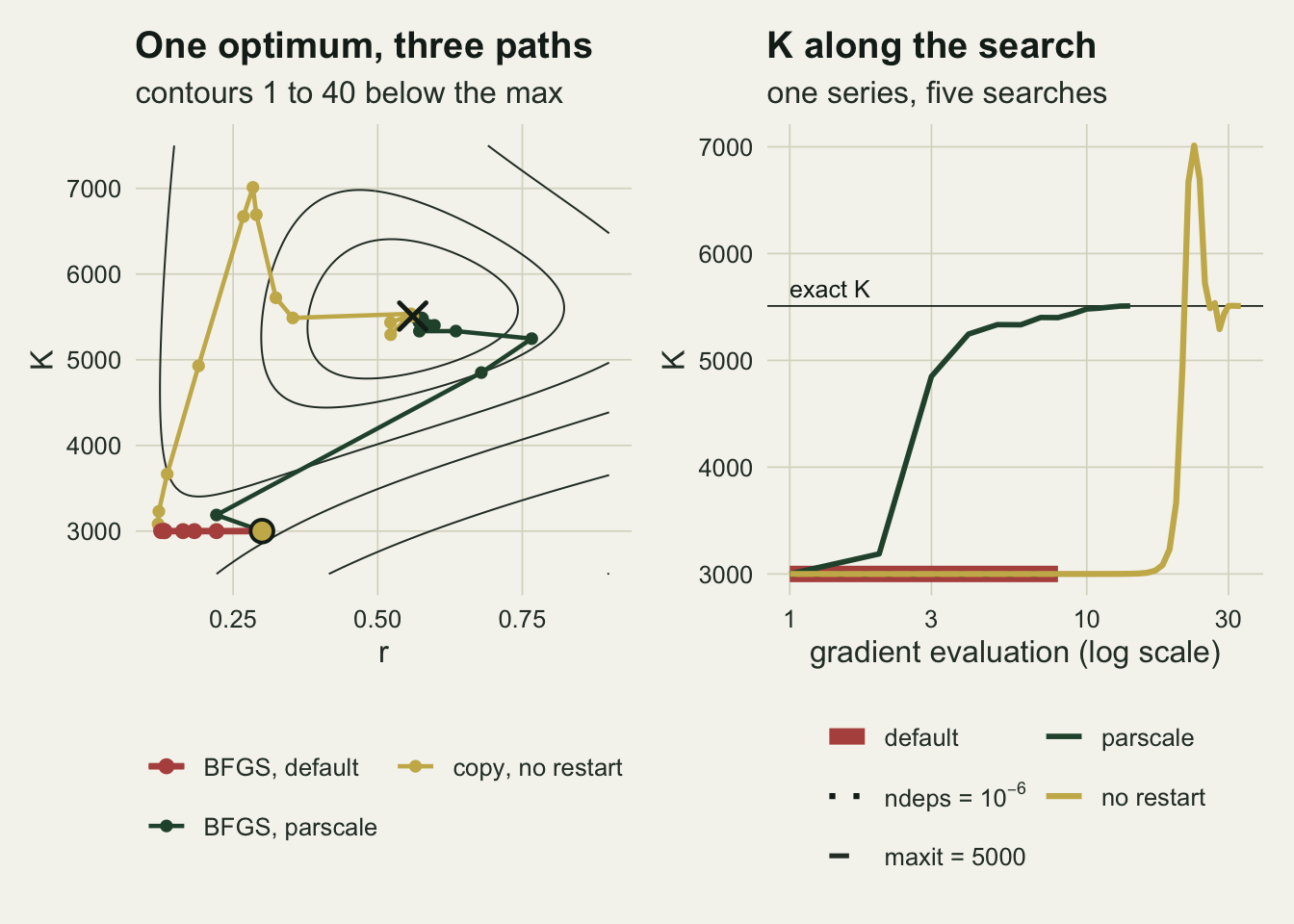
What L-BFGS-B and nlminb do differently
L-BFGS-B also works from a finite-difference gradient with the same ndeps, so if the gradient were the problem it would fail too. It mostly does not. Its design is described by Byrd and colleagues 1995, and it differs from optim()’s BFGS in two ways that can be measured from outside. It keeps its last five pairs of steps and gradient changes (lmm = 5) and rebuilds its matrix from them at each iteration, instead of discarding what it has learned on a schedule. And its default stopping rule, factr = 1e7, asks for a relative reduction of about \(2.2 \times 10^{-9}\) per iteration, which is about seven times tighter than the reltol of about \(1.5 \times 10^{-8}\) that BFGS uses. The question a numerical analyst would ask first is whether the box bounds help, since a box can rescale the problem as a side effect. The no-box calls answer that, and one more call, L-BFGS-B without a box and with factr = 1e8, puts its tolerance within a factor of two of BFGS’s.
stuck_lb  <- mean(stuck(res_far, "lb"));  stuck_lbn <- mean(stuck(res_far, "lbn"))
off_def <- share_off(res_far, "def")
off_lb  <- share_off(res_far, "lb");      off_lbn <- share_off(res_far, "lbn")
code0_stuck_all <- mean(c(res_far["code", "lb", stuck(res_far, "lb")],
                          res_far["code", "lbn", stuck(res_far, "lbn")]) == 0)
off_is_stuck <- mean(stuck(res_far, "lbn")[abs(rel_err(res_far, "lbn")) > 0.10])
stuck_def <- mean(stuck(res_far, "def"))
tol_lb  <- 1e7 * .Machine$double.eps / sqrt(.Machine$double.eps)   # factr tolerance over reltol
res_lb8 <- vapply(fms, function(fm) one_row(optim(start_far, fm$nll_K, method = "L-BFGS-B",
                                           control = list(factr = 1e8))), numeric(3))
err_lb8   <- abs(res_lb8["K", ] - K_ex) / K_ex
off_lb8   <- mean(err_lb8 > 0.10)
code0_lb8 <- mean(res_lb8["code", err_lb8 > 0.10] == 0)
With the box, L-BFGS-B leaves 0.058 of the series more than ten per cent off; without it, 0.108. So the box helps a little and is not what makes the method work. The misses are not near misses either. A fit counts as stuck here if its K ended within a tenth of a per cent of the starting 3000, and 0.058 of the boxed fits and 0.108 of the unboxed ones are stuck; every unboxed fit more than ten per cent off is a stuck one (share 1.00). The stuck fits report code 0 in 1.00 of cases. When L-BFGS-B fails, it fails the way BFGS fails, only less often: it settles r and sigma for the starting K and stops with a clean code. For comparison, 0.356 of the default BFGS fits are stuck by the same definition.
The tolerance is a large part of the rest. The default factr is 6.71 times tighter than BFGS’s reltol; loosen it tenfold, to factr = 1e8, and 0.548 of the unboxed fits are more than ten per cent off, 1.00 of those with code 0. What remains of L-BFGS-B’s advantage at a comparable tolerance is consistent with its not restarting, but its source was not stepped through here, so that part is an inference from the design and not a measurement.
nlminb(), which calls the PORT library, is exact in all 500 series with and without bounds. That is a measurement on this model, not a property to rely on: the practical lesson from L-BFGS-B is that two methods of the same family, each called with its own defaults, can differ 17-fold in how often they miss by more than a tenth, so no rule of thumb about “gradient methods” settles it for a given fit.
A careful start shrinks the error, not the problem
The size of the failure depends on the start. A start of K = 3000 when the answer is near 5000 is a plausible guess, but a careful analyst would start from the data. Here is a moment-based start, written before it was run: K from the mean of the second half of the series, when the colony should be fluctuating around its ceiling, and r from the mean log growth over the first five years divided by one minus the mean relative density over those years, kept between 0.05 and 1.5. Sigma starts at 0.3 as before.
moment_start <- function(N) {
  K0 <- mean(N[(n_yr / 2 + 1):n_yr])
  g5 <- diff(log(N))[1:5]
  r0 <- mean(g5) / (1 - mean(N[1:5]) / K0)
  c(min(max(r0, 0.05), 1.5), K0, log(0.3))
}
starts_m <- lapply(series, moment_start)
K_start_m <- vapply(starts_m, function(s) s[2], 0)
res_mom <- vapply(seq_along(fms), function(i)
  run_fitters(fms[[i]], starts_m[[i]], which = c("def", "maxit", "pars")),
  matrix(0, 3, 3))
dimnames(res_mom)[[2]] <- c("def", "maxit", "pars")
tab_mom <- do.call(rbind, lapply(c("def", "maxit", "pars"), function(f) summ(res_mom, f)))
start_err_m <- (K_start_m - K_ex) / K_ex
travel <- function(res, f, K0) (res["K", f, ] - K0) / (K_ex - K0)
trav_far <- median(travel(res_far, "def", start_far[2]))
trav_mom <- median(travel(res_mom, "def", K_start_m))
trav_mom_mx <- median(travel(res_mom, "maxit", K_start_m))
code0_mom <- share_code0(res_mom, "def"); code0_mom_mx <- share_code0(res_mom, "maxit")
From the moment start the default BFGS call is a median 4.3 to 5.9 per cent from the exact K per block, and 0.15 of all series are more than ten per cent off. The moment start itself is a median 5.4 per cent from the exact K. That is the number to read next to the fit’s error: the fit is barely better than its own start. The fraction of the distance from the starting K to the exact K that the default call covers is a median 0.011 from the far start and 0.004 from the moment start; with maxit = 5000 from the moment start it is 0.022. Code 0 is reported in 0.51 of the default fits and 0.82 with the raised limit. parscale from the moment start is exact again: its largest error in K over all 500 series is 0.00017.
So the careful start makes the headline smaller and the problem no smaller: BFGS in (r, K) returns something close to the K it was given. A good start hides that, because the answer looks sensible; it does not make the search find anything.
st_df <- rbind(
  data.frame(start = "far start, K = 3000", call = "BFGS, default",
             x = (start_far[2] - K_ex) / K_ex, y = rel_err(res_far, "def")),
  data.frame(start = "moment start", call = "BFGS, default",
             x = start_err_m, y = rel_err(res_mom, "def")),
  data.frame(start = "far start, K = 3000", call = "BFGS, parscale",
             x = (start_far[2] - K_ex) / K_ex, y = rel_err(res_far, "pars")),
  data.frame(start = "moment start", call = "BFGS, parscale",
             x = start_err_m, y = rel_err(res_mom, "pars")))
ggplot(st_df, aes(x, y, colour = call)) +
  geom_abline(slope = 1, intercept = 0, colour = te_body, linetype = "dashed", linewidth = 0.5) +
  geom_hline(yintercept = 0, colour = te_ink, linewidth = 0.4) +
  geom_point(size = 1.1, alpha = 0.6) +
  facet_wrap(~ start, scales = "free_x") +
  scale_colour_manual(values = c(te_rust, te_forest), name = NULL) +
  scale_x_continuous(labels = pct) + scale_y_continuous(labels = pct) +
  labs(x = "starting K relative to the exact MLE", y = "fitted K relative to the exact MLE",
       title = "BFGS in (r, K) hands back its starting K",
       subtitle = "dashed diagonal: the fit returned its start") +
  theme_datasheet() + theme(legend.position = "bottom",
                            strip.text = element_text(colour = te_ink, face = "bold"))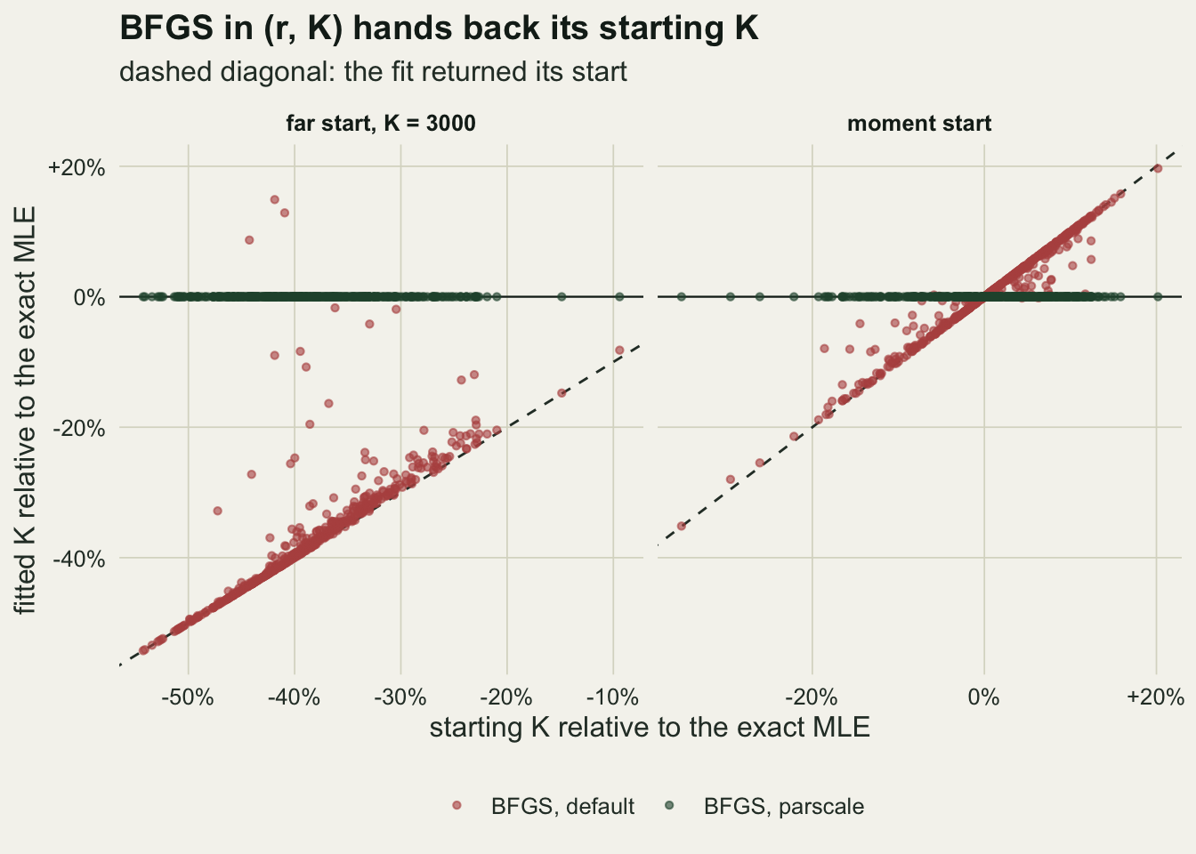
Look for the linear form first
The honest ordering of repairs starts before optim(). This model is a linear regression in (r, b), and a reader who noticed that would never have met any of the above; lm() gives the maximum, its standard errors, and K as a ratio whose interval can be had by the delta method or by profiling. Many ecological models are not linear in any spelling, and for those the order is: put every parameter on a scale where one unit is a meaningful change, either by rescaling the parameter itself (K in thousands, or log K, as the theta-logistic post does) or by passing parscale with the rough size of each parameter; then check the answer against a second method that does not share the first one’s weakness. Nelder-Mead and nlminb() were exact here from a bad start, and a disagreement between two fitters is information that a convergence code never carries. Bolker 2008 treats this kind of fitting at length for ecological models; Nash 2014 is the book on what the R optimisers do inside.
The two rescalings are cheap to check on the same series and from the same start, with the plain BFGS call and nothing in the control list.
res_logK <- vapply(fms, function(fm) {
  o <- optim(c(start_far[1], log(start_far[2]), start_far[3]),
             function(th) fm$nll_K(c(th[1], exp(th[2]), th[3])), method = "BFGS")
  c(K = exp(o$par[2]), code = o$convergence) }, numeric(2))
res_kK <- vapply(fms, function(fm) {
  o <- optim(c(start_far[1], start_far[2] / 1000, start_far[3]),
             function(th) fm$nll_K(c(th[1], 1000 * th[2], th[3])), method = "BFGS")
  c(K = 1000 * o$par[2], code = o$convergence) }, numeric(2))
err_logK <- abs(res_logK["K", ] - K_ex) / K_ex
err_kK   <- abs(res_kK["K", ] - K_ex) / K_ex
In log K the largest relative error in K over all 500 series is 0.00013, and with K in thousands it is 0.000059; both calls report code 0 in a share of 1.000 and 1.000 of series. Either spelling gives the restart an identity matrix of about the right shape to return to.
?optim documents parscale accurately, and it is still not a matter of reading the help page, for two reasons. The failing call is the plain one, optim(start, nll, method = "BFGS"), with no control list at all, and the output either says it converged or gives a code 1 that a raised maxit often removes. And the obvious neighbouring methods do not agree: L-BFGS-B, with its own tighter default tolerance, mostly succeeds from the same start, so a reader who had once switched methods and seen the problem go away would have learned the wrong lesson.
What to report
State the parameterisation that was optimised, not only the one reported. A carrying capacity reported from a fit in log K and one from a fit in K are the same number only when both searches reached the maximum.
Report the optimiser, the start and the control list, including any parscale or rescaling. A reader who can see method = "BFGS" with a K in the thousands and no scaling now knows what to check.
Report the log-likelihood at the answer, and where possible the log-likelihood from a second fitter or a second start. Here the default fits fell a median 4.62 to 4.99 units short of the maximum per block, which is a difference a second fit would have shown immediately and a convergence code never did.
Do not report convergence code 0 as evidence that the maximum was found. In this model it was reported by 61 per cent of fits with a raised iteration limit, most of them wrong by more than a tenth of K.
Honest limits
The size of the failure is a function of how far the start is from the maximum, and most of the headline numbers here are for one fixed start. The moment-based arm is the check on that: it shrinks the error to roughly the error of the start itself. The finding that survives both starts is the fraction of the distance travelled, not the size of the error.
This is one model with three parameters, one of them thousands of times larger than the others. The same mechanism applies to any parameter whose gradient is small next to its neighbours’, such as a home-range scale in metres, an asymptotic length in millimetres or a population size, but the size of the effect in those models was not measured here. Rescaling every parameter to order one removes this particular failure when the gradient is of order one as well; a parameter near one that multiplies a covariate measured in thousands is badly scaled in the same way.
Only one noise level, one series length and one true growth rate were run. A longer series or a noisier one changes the curvature of the likelihood and could change how far BFGS gets before its relative tolerance stops it. For BFGS the tolerance was varied in one arm only, a tighter reltol at the default iteration limit; the tighter tolerance combined with a raised limit was not run.
For BFGS the mechanism is measured: the R copy of vmmin reproduces optim() exactly, and deleting its restart line and nothing else makes every fit exact. For L-BFGS-B only part of it is: bounds are not what make it work, its tighter default tolerance accounts for much of its advantage, and when it fails it stops at its starting K. That the rest comes from not restarting is an inference from its published design, not a step through its source. nlminb() never failed here, and that is one model’s result, not a guarantee.
Finally, everything here is a demonstration of a known property of gradient methods, whose scaling Nash and Varadhan 2011 treat among the diagnostics for optim() and its relatives. The measured pieces are the size of the shortfall on an ordinary ecological fit, the rise in clean convergence codes under a raised maxit, and the tracing of the failure past the finite-difference step and the step length to the periodic restart in optim()’s BFGS code.
References
Nash JC, Varadhan R 2011 Journal of Statistical Software 43(9):1-14 (10.18637/jss.v043.i09)
Nelder JA, Mead R 1965 Computer Journal 7(4):308-313 (10.1093/comjnl/7.4.308)
Byrd RH, Lu P, Nocedal J, Zhu C 1995 SIAM Journal on Scientific Computing 16(5):1190-1208 (10.1137/0916069)
Ricker WE 1954 Journal of the Fisheries Research Board of Canada 11(5):559-623 (10.1139/f54-039)
Nash JC 2014 Nonlinear Parameter Optimization Using R Tools (ISBN 978-1-118-56928-3)
Bolker BM 2008 Ecological Models and Data in R (ISBN 978-0-691-12522-0)