library(lme4)
library(ggplot2)

te_paper  <- "#f5f4ee"
te_ink    <- "#16241d"
te_body   <- "#2c3a31"
te_forest <- "#275139"
te_rust   <- "#b5534e"
te_gold   <- "#c9b458"
te_line   <- "#dad9ca"

theme_datasheet <- function() {
  theme_minimal(base_size = 12) +
    theme(plot.background  = element_rect(fill = te_paper, colour = NA),
          panel.background = element_rect(fill = te_paper, colour = NA),
          panel.grid.major = element_line(colour = te_line, linewidth = 0.3),
          panel.grid.minor = element_blank(),
          text             = element_text(colour = te_body),
          plot.title       = element_text(colour = te_ink, face = "bold"),
          plot.subtitle    = element_text(colour = te_body),
          axis.text        = element_text(colour = te_body),
          strip.text       = element_text(colour = te_ink))
}
The lme4 max|grad| warning and predictor scale
R
mixed models
lme4
GLMM
simulation
ecology tutorial
Raw calendar year in a glmer sets off the max|grad| warning. Measuring in R when the estimates are fine, when the standard error is not, and which check to run.
Twenty springs of territory counts of a woodland warbler in fifteen woods, 2001 to 2020, and for each wood its distance from the nearest main road in metres. The model is the one every course teaches for this design: a Poisson GLMM with a random intercept for wood, fitted with glmer(), with year and distance entered exactly as they sit in the spreadsheet. The fit comes back with estimates and three messages. One begins Model failed to converge with max|grad| =, followed by a number, the tolerance 0.002 and a component number; the other two say the model is nearly unidentifiable and end in Rescale variables?.
Two replies to that warning circulate. One says it is a known false positive and can be ignored; the other says to swap optimisers until it goes away. Both treat it as a property of the optimiser. This post measures what the warning is attached to: whether the estimates, the standard errors and the likelihood of the fit that carries it are right. The measuring stick is the same model refitted with the predictors centred and rescaled, which leaves the likelihood unchanged and changes only the arithmetic.
The mirror image of the problem is already on this site. Parameter scale decides what optim() finds shows optim() returning convergence code 0 on a carrying capacity more than a tenth out, and in its section on repairs gives the advice to rescale and then check the answer against a second method that does not share the first one’s weakness. Here the flag goes up on a fit whose estimate is right, and the second method most people reach for, allFit(), can share the weakness that matters. Random slopes in mixed models with nlme tells the reader to centre the predictor so that the intercept variance and the intercept-slope correlation mean something; below, with a random slope for year, centring decides whether the fit reaches its maximum at all. Pseudoreplication: GLMMs for nested counts in R fits glmer() to predictors simulated as standard normal variables, which is the coding every fit here is checked against. Random effects with too few levels treats a singular fit as a report about the data; here the same message turns up on fits that have simply stopped short of the maximum. And AIC on REML fits: when units choose the model shows elevation in metres or kilometres changing the REML likelihood itself, which is a different effect of units: in the models below the likelihood does not depend on the units at all.
One survey, four codings
The generating model has a log mean count of 1 at the centre of the study, a wood effect with standard deviation 0.6 on the log scale, a decline of 0.3 per decade and a rise of 0.25 per kilometre of distance from the road. Each wood gets one distance, drawn between 50 and 3000 m. The survey data frame carries the two predictors in four codings: raw (calendar year, metres), centred (years from 2010.5, metres from 1500), rescaled but not centred (decades since year zero, kilometres) and both (decades from 2010.5, kilometres from 1500).
n_year <- 20; years <- 2001:2020
b0 <- 1; b_dec <- -0.3; b_km <- 0.25; sd_wood <- 0.6
year_mid <- 2010.5; dist_mid <- 1500

make_survey <- function(n_wood, sd_slope = 0) {
  wood <- factor(rep(seq_len(n_wood), each = n_year))
  year <- rep(years, n_wood)
  dist <- rep(runif(n_wood, 50, 3000), each = n_year)          # metres
  u0 <- rnorm(n_wood, 0, sd_wood); u1 <- rnorm(n_wood, 0, sd_slope)
  dec <- (year - year_mid) / 10; km <- (dist - dist_mid) / 1000
  count <- rpois(n_wood * n_year, exp(b0 + u0[wood] + (b_dec + u1[wood]) * dec + b_km * km))
  data.frame(count, wood, year, dist,
             year_c = year - year_mid, dist_c = dist - dist_mid,  # centred
             year_d = year / 10, dist_k = dist / 1000,            # rescaled
             dec, km)                                             # both
}

# every warning and message is captured, none is printed
fit_log <- function(expr) { said <- character(0)
  fit <- withCallingHandlers(expr,
    warning = function(w) { said <<- c(said, conditionMessage(w)); invokeRestart("muffleWarning") },
    message = function(m) { said <<- c(said, conditionMessage(m)); invokeRestart("muffleMessage") })
  list(fit = fit, said = said, conv = unlist(fit@optinfo$conv$lme4$messages)) }
vcov_log <- function(fit) { fell <- FALSE
  v <- withCallingHandlers(vcov(fit), warning = function(w) { fell <<- TRUE; invokeRestart("muffleWarning") })
  list(v = as.matrix(v), fell = fell) }
has <- function(txt, pattern) any(grepl(pattern, txt, fixed = TRUE))
grad_of <- function(conv) { g <- regmatches(conv, regexpr("max\\|grad\\| = [0-9.e+-]+", conv))
  if (length(g)) as.numeric(sub(".*= ", "", g[1])) else NA_real_ }
All four codings describe one model. Each is an affine change of the fixed-effect columns, which maps the fixed coefficients onto each other by a known linear transformation and leaves the random intercept and the maximised likelihood where they were. Any difference between the four fits is therefore numerical. The rates below are read from the messages lme4 stores in the fit object (fit@optinfo$conv$lme4$messages), not from console text; the one message lme4 raises before fitting, about predictor scales, is captured as a condition when the model is built.
set.seed(2610)
n_tries <- 0
repeat {                     # first survey whose raw fit carries the warning
  n_tries <- n_tries + 1
  woods <- make_survey(15)
  raw_w <- fit_log(glmer(count ~ year + dist + (1 | wood), family = poisson, data = woods))
  if (has(raw_w$conv, "max|grad|")) break
}
both_w <- fit_log(glmer(count ~ dec + km + (1 | wood), family = poisson, data = woods))
writeLines(raw_w$conv)
Model failed to converge with max|grad| = 0.0170357 (tol = 0.002, component 1)
See ?lme4::convergence and ?lme4::troubleshooting.
Model is nearly unidentifiable: very large eigenvalue
- Rescale variables?
Model is nearly unidentifiable: large eigenvalue ratio
- Rescale variables?length(both_w$conv)[1] 0w_grad <- grad_of(raw_w$conv)
w_b <- c(raw = fixef(raw_w$fit)[["year"]] * 10, both = fixef(both_w$fit)[["dec"]])
w_km <- c(raw = fixef(raw_w$fit)[["dist"]] * 1000, both = fixef(both_w$fit)[["km"]])
w_dll <- as.numeric(logLik(both_w$fit) - logLik(raw_w$fit))
w_sd <- c(raw = attr(VarCorr(raw_w$fit)$wood, "stddev")[[1]],
both = attr(VarCorr(both_w$fit)$wood, "stddev")[[1]])
w_se <- c(raw = sqrt(vcov_log(raw_w$fit)$v[2, 2]) * 10, both = sqrt(vcov_log(both_w$fit)$v[2, 2]))
w_se_rx <- sqrt(as.matrix(suppressWarnings(vcov(both_w$fit, use.hessian = FALSE)))[2, 2])
# summary() prints the standard errors that vcov() returns by default,
# which for a glmer fit use the finite-difference Hessian when it exists
se_summary <- suppressWarnings(coef(summary(raw_w$fit))[, "Std. Error"])
se_hess <- sqrt(diag(as.matrix(suppressWarnings(vcov(raw_w$fit, use.hessian = TRUE)))))
stopifnot(isTRUE(all.equal(unname(se_summary), unname(se_hess))))The first survey drawn gives the raw fit the warning, with max|grad| at 0.0170, together with both identifiability messages; the fit in centred and rescaled units carries none. The estimates agree. The decline is -0.28186 per decade from the raw fit and -0.28186 from the other, the distance effect 0.34876 and 0.34877 per kilometre, the wood standard deviation 0.54930 and 0.54929, and the log-likelihoods differ by \(1.6 \times 10^{-9}\). The standard error of the decline is 0.0506 per decade from the raw fit and 0.0510 from the centred one, which in this survey is also agreement. Keep that last comparison in mind: it is the one that changes from survey to survey.
What the check computes
After the optimiser stops, lme4 estimates the gradient and the Hessian of the deviance at the returned point by finite differences. For a glmer() fit with the default Laplace approximation the parameters are the wood standard deviation (strictly the relative covariance factor theta of Bates and colleagues 2015, which for a Poisson random intercept is the standard deviation) and the three fixed effects together. It then forms a scaled gradient, the gradient premultiplied by the inverse of the Cholesky factor of the Hessian, takes the smaller of the scaled and the raw absolute gradient for each parameter, and warns if the largest of those exceeds a tolerance of 0.002. Both stages of the default glmer() optimisation are derivative free (bobyqa, then the Nelder and Mead 1965 simplex), so this finite-difference gradient is the first derivative of the deviance with respect to the optimised parameters that is ever computed.
cc <- glmerControl()$checkConv$check.conv.grad
stopifnot(cc$action == "warning", cc$tol == 0.002,
          identical(glmerControl()$optimizer, c("bobyqa", "Nelder_Mead")))

min_grad <- function(der) pmin(abs(solve(chol(der$Hessian), der$gradient)), abs(der$gradient))
der_raw  <- raw_w$fit@optinfo$derivs
der_both <- both_w$fit@optinfo$derivs
mg_raw   <- min_grad(der_raw)
stopifnot(abs(max(mg_raw) / w_grad - 1) < 1e-4)     # the message prints six digits
par_lab  <- c("wood SD", "intercept", "year", "distance")
top_par  <- par_lab[which.max(mg_raw)]
comp_msg <- as.integer(sub(".*component ([0-9]+).*", "\\1",
                           raw_w$conv[grepl("max|grad|", raw_w$conv, fixed = TRUE)]))
cond_no  <- function(der) { ev <- eigen(der$Hessian, symmetric = TRUE, only.values = TRUE)$values; max(ev) / min(ev) }
kap <- c(raw = cond_no(der_raw), both = cond_no(der_both))

scalex_tol <- formals(getFromNamespace("checkScaleX", "lme4"))$tol
stopifnot(scalex_tol == 1000)
sd_pred <- c(year = sd(woods$year), dist = sd(woods$dist))
Rebuilt from the stored derivatives, the largest of those minima is 0.0170, the number in the message, and it belongs to the year coefficient. The message nevertheless says component 1. In the installed lme4 (2.0.1), and in the current source on GitHub, the component is computed as which.max() of the maximum, a single number, so it is always 1; the component number in this message carries no information.
The Hessian says why the check is struggling. Its condition number, the ratio of the largest to the smallest eigenvalue, is about 32 billion in raw units and 22 after centring and rescaling. The calendar year sits more than two thousand units from zero and moves by nineteen, so the intercept (the log count in year zero) and the year coefficient are almost perfectly confounded, and the deviance is extremely steep along one combination of them and nearly flat along another. A finite difference with one step size cannot get both right. The optimiser has found the maximum; the arithmetic used to check it and to compute the curvature is what fails.
lme4 has a separate check for predictor scale, run when the model is built. It warns Some predictor variables are on very different scales: consider rescaling when a continuous predictor has a standard deviation above 1000 or below 1/1000, or when two standard deviations differ by more than a factor of 1000 (the threshold is 1000 in the source). It looks only at standard deviations. In this survey year has a standard deviation of 5.78 and distance 606 m, so it stays silent; the offset of the calendar year from zero, which is the actual problem, is invisible to it.
A hundred and sixty surveys at three sizes
The worked survey is one draw. The simulation below repeats it with 15, 60 and 240 woods (300, 1200 and 4800 counts), fitting all four codings to every survey, and compares each coding with the centred and rescaled fit. The replicate counts, 100, 40 and 20 surveys, were fixed before any rate was looked at; the larger designs cost more per fit.
codings <- list(raw = c("year", "dist"), centred = c("year_c", "dist_c"),
                rescaled = c("year_d", "dist_k"), both = c("dec", "km"))
per_dec <- c(raw = 10, centred = 10, rescaled = 1, both = 1)
cod_lev <- names(codings)

one_survey <- function(d) {
  out <- do.call(rbind, lapply(cod_lev, function(k) {
    f <- fit_log(glmer(reformulate(c(codings[[k]], "(1 | wood)"), "count"),
                       family = poisson, data = d))
    vc <- vcov_log(f$fit)
    comp <- if (has(f$conv, "max|grad|"))
      as.integer(sub(".*component ([0-9]+).*", "\\1", f$conv[grepl("max|grad|", f$conv, fixed = TRUE)][1]))
      else NA_integer_
    data.frame(coding = k, warn = has(f$conv, "max|grad|"), grad = grad_of(f$conv),
               comp = comp, hess = has(f$conv, "Rescale variables"),
               scalex = has(f$said, "very different scales"), sing = isSingular(f$fit),
               fell = vc$fell, ll = as.numeric(logLik(f$fit)),
               b = unname(fixef(f$fit)[2]) * per_dec[[k]], se = sqrt(vc$v[2, 2]) * per_dec[[k]],
               se_rx = sqrt(as.matrix(suppressWarnings(vcov(f$fit, use.hessian = FALSE)))[2, 2]) * per_dec[[k]],
               sd_w = attr(VarCorr(f$fit)$wood, "stddev")[[1]])
  }))
  ref <- out[out$coding == "both", ]
  out$se_ratio <- out$se / ref$se; out$rx_ratio <- out$se_rx / ref$se; out$db <- out$b - ref$b
  out$dll <- out$ll - ref$ll; out$dsd <- out$sd_w - ref$sd_w
  out$sd_dist <- sd(d$dist)
  out
}

n_rep <- c("15" = 100, "60" = 40, "240" = 20)     # fixed before running
set.seed(3107)
small_surveys <- list()
sims <- do.call(rbind, lapply(names(n_rep), function(jj) {
  do.call(rbind, lapply(seq_len(n_rep[[jj]]), function(i) {
    d <- make_survey(as.integer(jj))
    if (jj == "15") small_surveys[[i]] <<- d
    cbind(n_wood = as.integer(jj), n_obs = as.integer(jj) * n_year, rep = i, one_survey(d))
  }))
}))
sims$coding <- factor(sims$coding, levels = cod_lev)
sims$off <- abs(sims$se_ratio - 1) > 0.1

rate_tab <- aggregate(cbind(warn, hess, scalex, sing, fell, off) ~ coding + n_obs, data = sims, FUN = mean)
rate_tab$n <- n_rep[as.character(rate_tab$n_obs / n_year)]
rate_of <- function(col, k, n) rate_tab[[col]][rate_tab$coding == k & rate_tab$n_obs == n]
obs_lev <- sort(unique(sims$n_obs))
mcse <- function(p, n) sqrt(p * (1 - p) / n)

raw_s <- sims[sims$coding == "raw", ]
max_db  <- max(abs(sims$db)); max_dll <- max(abs(sims$dll)); max_dsd <- max(abs(sims$dsd))
med_grad <- tapply(raw_s$grad, raw_s$n_obs, median, na.rm = TRUE)
comp_all_one <- all(sims$comp[!is.na(sims$comp)] == 1)
stopifnot(comp_all_one)
in_m <- sims$coding %in% c("raw", "centred")             # distance still in metres
scalex_rule <- all(sims$scalex[in_m] == (sims$sd_dist[in_m] > scalex_tol)) && !any(sims$scalex[!in_m])
n_scalex <- sum(raw_s$scalex)
se_q <- function(k, n, p) quantile(sims$se_ratio[sims$coding == k & sims$n_obs == n], p, names = FALSE)
n_fell <- sum(sims$fell)
Across all 640 fits the four codings return the same estimates. The largest difference from the centred and rescaled fit is \(1.4 \times 10^{-4}\) per decade in the decline, \(1.6 \times 10^{-5}\) in the wood standard deviation and \(3.1 \times 10^{-6}\) in the log-likelihood. The warning is another matter.
With 300 counts the raw fit carries the max|grad| warning in 98 per cent of surveys, with 1200 in 100 per cent and with 4800 in 100 per cent. Centring alone, with distance still in metres, brings the rate down to 3, 5 and 20 per cent; rescaling without centring leaves it at 75, 62 and 80 per cent; doing both removes it from every survey. The identifiability message ending in Rescale variables? appears in every fit in the first three codings and in 0 per cent of the centred and rescaled ones, so lme4 does point at scale in every raw fit, through this message rather than through its dedicated scale check. The construction-time scale message, very different scales, appears in 5 of the 160 raw fits, each time in a survey whose woods have a distance standard deviation above 1000 m; the year never sets it off.
The warning rate does not grow with the number of counts in this design, because it is already near its ceiling at the smallest one. The number printed in it is larger at the largest size: the median max|grad| of the raw fits is 0.034, 0.037 and 0.070 at the three sizes. Every one of the 283 warnings names component 1.
rate_tab$mc <- mcse(rate_tab$warn, rate_tab$n)
ggplot(rate_tab, aes(n_obs, warn, colour = coding)) +
  geom_errorbar(aes(ymin = pmax(0, warn - 2 * mc), ymax = pmin(1, warn + 2 * mc)),
                width = 0.05, linewidth = 0.4) +
  geom_line(linewidth = 0.9) + geom_point(size = 2.4) +
  scale_x_log10(breaks = obs_lev) +
  scale_y_continuous(limits = c(0, 1)) +
  scale_colour_manual(values = c(te_rust, te_gold, te_body, te_forest), name = NULL) +
  labs(x = "counts in the survey (log scale)", y = "share of fits with the warning",
       title = "The warning follows the coding, not the data",
       subtitle = "same model, same surveys, four codings of year and distance") +
  theme_datasheet() + theme(legend.position = "bottom")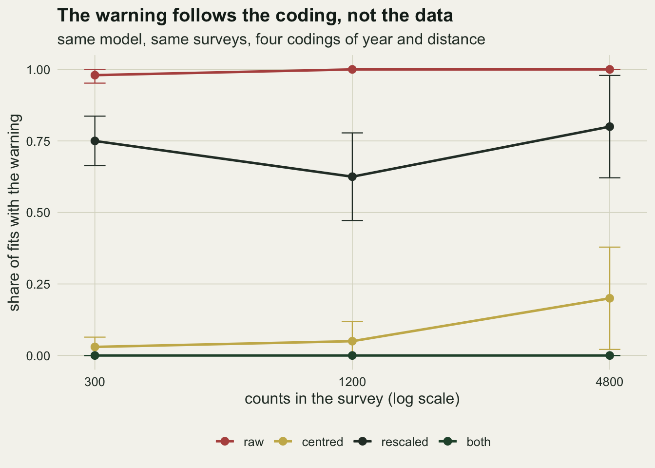
The standard error is where the raw fit goes wrong
The same finite-difference Hessian that feeds the check also feeds the standard errors. For a glmer() fit summary() prints the ones vcov() returns by default, and that default inverts the finite-difference Hessian whenever one was computed (the chunk above checks that equality on the worked fit). An inaccurate Hessian does not move the estimate, which the optimiser found without it, but it moves every Wald test and interval built on it.
off_rate <- function(k, n) rate_of("off", k, n)
lo_raw <- se_q("raw", 300, c(0, 0.1, 0.5))
worst_raw <- min(sims$se_ratio[sims$coding == "raw"])
other_worst <- max(abs(sims$se_ratio[sims$coding %in% c("centred", "rescaled")] - 1))
one_way <- all(sims$se_ratio[sims$coding == "raw" & sims$off] < 1)
n_off_raw <- sum(sims$coding == "raw" & sims$off)
n_small <- sum(sims$coding == "raw" & sims$off & sims$se_ratio < 1)

# coverage of the true decline by the 95 per cent Wald interval, 300 counts
s3 <- sims[sims$n_obs == 300, ]
off3 <- s3$off[s3$coding == "raw"]
cover <- function(k, rows = TRUE)
  mean((abs((s3$b[s3$coding == k] - b_dec) / s3$se[s3$coding == k]) < qnorm(0.975))[rows])
cov_ref <- cover("both"); cov_raw <- cover("raw")
# standard errors from the fixed-effect model matrix instead of the Hessian
rx_worst <- max(abs(sims$rx_ratio - 1))
raw_flag <- abs(raw_s$se / raw_s$se_rx - 1) > 0.1
flag_match <- all(raw_flag == raw_s$off)
With 300 counts the standard error of the decline from the raw fit is more than ten per cent away from the centred and rescaled one in 35 per cent of surveys (Monte Carlo standard error 5 points). Over those 100 surveys the ratio of the two standard errors has a minimum of 0.11, a tenth percentile of 0.23 and a median of 0.98: the raw fit usually reports the right uncertainty and, a good part of the time, an uncertainty several times too small. Every one of the wrong standard errors is too small, so the error runs one way, towards overconfidence. With 1200 and 4800 counts the share falls to 0 and 0 per cent, so the larger surveys keep the warning and lose the damage. Centring alone or rescaling alone never moves the standard error by more than 9 per cent in any survey. In none of the fits did vcov() fall back to the other estimate of the covariance, the one built from the fixed-effect model matrix; the wrong standard errors come from a Hessian that was positive definite, so vcov() used it without comment, although lme4 had already called it nearly unidentifiable. That other estimate, which vcov(fit, use.hessian = FALSE) returns on request, does not use the Hessian at all: in every fit of every coding it stays within 0.5 per cent of the reference, and on the raw fits it differs from the default standard error by more than ten per cent in exactly the surveys whose standard error was off.
The simulation also knows the true decline, 0.3 per decade, so the reference does not have to be taken on trust. With 300 counts the 95 per cent Wald interval from the centred and rescaled fit covers the true decline in 96 per cent of surveys and the one from the raw fit in 76 per cent (Monte Carlo standard errors 2 and 4 points). In the 35 surveys whose raw standard error was off, the two intervals cover it in 94 and 37 per cent, so it is the raw standard errors that are wrong, and wrong on the small side.
se_plot <- sims[sims$coding != "both", ]
se_plot$size_lab <- factor(sprintf("%d counts", se_plot$n_obs), levels = sprintf("%d counts", obs_lev))
set.seed(11)
ggplot(se_plot, aes(coding, se_ratio, colour = coding)) +
  annotate("rect", xmin = -Inf, xmax = Inf, ymin = 0.9, ymax = 1.1, fill = te_line, alpha = 0.6) +
  geom_hline(yintercept = 1, colour = te_body, linetype = "dashed", linewidth = 0.5) +
  geom_jitter(width = 0.18, height = 0, size = 1.6, alpha = 0.8) +
  facet_wrap(~ size_lab) +
  scale_y_log10(breaks = c(0.1, 0.2, 0.5, 1, 2)) +
  scale_colour_manual(values = c(te_rust, te_gold, te_body), guide = "none") +
  labs(x = NULL, y = "standard error ratio (log scale)",
       title = "Right estimate, wrong standard error",
       subtitle = "raw calendar year with 300 counts reports too little uncertainty") +
  theme_datasheet()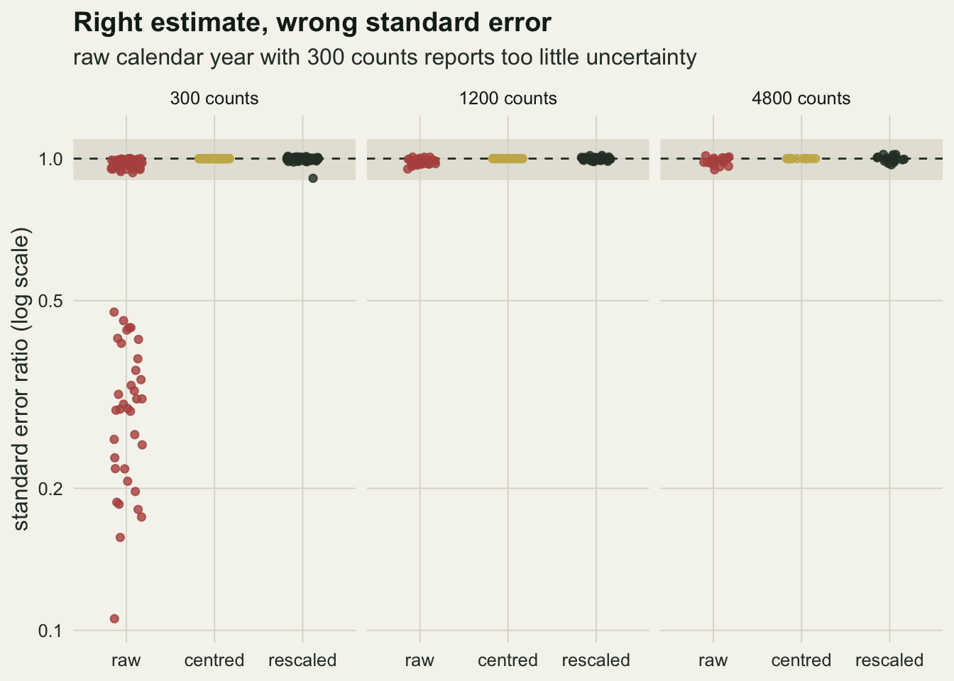
allFit agrees with itself
The standard advice for this warning is allFit(), which refits the model with every available optimiser and lets the user compare. Here it is run with the five optimisers lme4 provides without extra packages, on the small surveys in which the raw standard error was more than ten per cent off, up to the first twelve of them.
opt_tab <- cbind(optimizer = c("bobyqa", "Nelder_Mead", "nlminbwrap", "nloptwrap", "nloptwrap"),
                 method    = c("", "", "", "NLOPT_LN_NELDERMEAD", "NLOPT_LN_BOBYQA"))
# lme4 1.1-38 and later start every optimiser from the original fit unless told not to
af_extra <- if ("start_from_mle" %in% names(formals(allFit))) list(start_from_mle = FALSE) else list()
raw_small <- sims[sims$coding == "raw" & sims$n_wood == 15, ]
off_ids <- head(raw_small$rep[raw_small$off], 12)
af <- do.call(rbind, lapply(off_ids, function(i) {
  d <- small_surveys[[i]]
  raw_fit <- fit_log(glmer(count ~ year + dist + (1 | wood), family = poisson, data = d))$fit
  # allFit() refits by re-evaluating the model call, and from lme4 1.1-38 it does so where the
  # local d of this function is not visible, so the data frame itself goes into the call
  raw_fit@call$data <- d
  ref_fit <- fit_log(glmer(count ~ dec + km + (1 | wood), family = poisson, data = d))$fit
  all_raw <- suppressWarnings(suppressMessages(
    do.call(allFit, c(list(raw_fit, meth.tab = opt_tab, verbose = FALSE, data = d), af_extra))))
  s <- summary(all_raw)
  data.frame(survey = i, optimiser = names(all_raw),
             dll = s$llik - as.numeric(logLik(ref_fit)),
             db = s$fixef[, "year"] * 10 - fixef(ref_fit)[["dec"]],
             se_ratio = vapply(all_raw, function(f) sqrt(vcov_log(f)$v[2, 2]) * 10, 0) /
                        sqrt(vcov_log(ref_fit)$v[2, 2]),
             warn = vapply(s$msgs, function(m) has(unlist(m), "max|grad|"), TRUE))
}))
af_spread <- tapply(af$se_ratio, af$survey, function(z) max(z) / min(z))
n_af <- length(off_ids)
n_tight <- sum(af_spread < 1.01)
n_all_off <- sum(tapply(af$se_ratio, af$survey, function(z) all(abs(z - 1) > 0.1)))
On all 12 surveys the five optimisers reach the same log-likelihood as the centred fit to within 0.0045 and the same decline to within \(4.8 \times 10^{-4}\) per decade, and every one of the 60 refits carries the warning. By the usual reading, five optimisers agreeing on the maximum means the warning is a false positive and the fit can be reported. In 10 of the 12 surveys the five standard errors also agree with each other to within one per cent, and in 11 all five are more than ten per cent away from the correct value. The optimisers differ in how they search, but every one of them hands back a point in raw units, and the covariance of every one is then computed by the same finite-difference Hessian in the same badly conditioned coordinates. allFit() tests the search; it cannot test that.
af$opt_lab <- sub("nloptwrap.NLOPT_LN_", "nlopt ", af$optimiser)
ggplot(af, aes(factor(survey), se_ratio, colour = opt_lab, shape = opt_lab)) +
  geom_hline(yintercept = 1, colour = te_body, linetype = "dashed", linewidth = 0.5) +
  geom_point(position = position_dodge(width = 0.7), size = 2.2, stroke = 0.9) +
  scale_shape_manual(values = c(16, 17, 15, 1, 4), name = NULL) +
  scale_y_continuous(limits = c(0, 1.1), breaks = seq(0, 1, 0.25)) +
  scale_colour_manual(values = c(te_forest, te_rust, te_gold, te_body, te_ink), name = NULL) +
  guides(colour = guide_legend(nrow = 2), shape = guide_legend(nrow = 2)) +
  labs(x = "survey", y = "standard error ratio",
       title = "Five optimisers, one wrong standard error",
       subtitle = "dashed line: the standard error from the centred and rescaled fit") +
  theme_datasheet() + theme(legend.position = "bottom")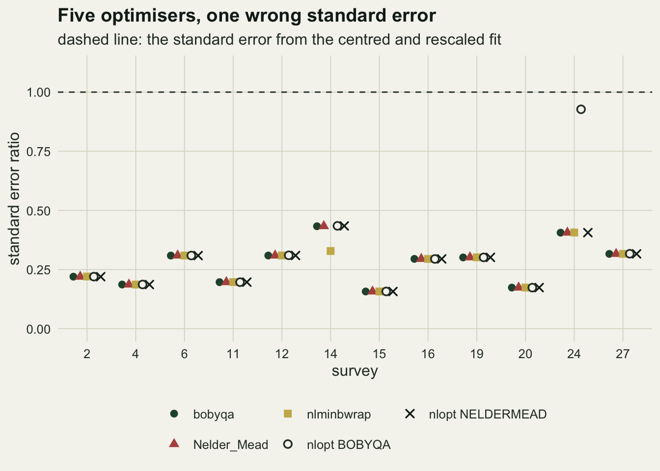
A fit the warning is right about
The raw-coded random intercept model always reached its maximum. Add the thing the analyst usually wants next, a random slope for year so that the trend can differ between woods, and that stops being true. The slope standard deviation in the simulation is 0.3 per decade, and the run is sixty surveys of fifteen woods, a count fixed in advance.
n_slope <- 60
sd_slope_set <- 0.3                                   # per decade
rho_implied <- -year_mid * sd_slope_set / 10 /
  sqrt(sd_wood^2 + (year_mid * sd_slope_set / 10)^2)  # year-zero intercept with slope
With calendar year as the covariate the random intercept is the log count in year zero, two thousand years outside the data, and the generating values imply a correlation of -0.99995 between that intercept and the slope. The model with (1 + year | wood) and the one with (1 + dec | wood) are still the same model, because an unstructured two by two covariance matrix maps onto itself under an affine change of the covariate, so their maximised likelihoods must be equal. Any fit that ends below the centred one has stopped at the wrong place.
msg_type <- function(conv) {
  if (has(conv, "singular")) "singular fit"
  else if (has(conv, "max|grad|")) "max|grad|"
  else if (has(conv, "degenerate") || has(conv, "unable to evaluate")) "degenerate Hessian"
  else if (length(conv)) "other message" else "no message"
}
set.seed(4419)
slope_surveys <- vector("list", n_slope); slope_raw_fits <- vector("list", n_slope)
sl <- do.call(rbind, lapply(seq_len(n_slope), function(i) {
  d <- make_survey(15, sd_slope = sd_slope_set)
  slope_surveys[[i]] <<- d
  fr <- fit_log(glmer(count ~ year + dist + (1 + year | wood), family = poisson, data = d))
  fs <- fit_log(glmer(count ~ dec + km + (1 + dec | wood), family = poisson, data = d))
  slope_raw_fits[[i]] <<- fr$fit
  data.frame(survey = i, gap = as.numeric(logLik(fs$fit) - logLik(fr$fit)), ll_ref = as.numeric(logLik(fs$fit)),
             se_rx_raw = sqrt(as.matrix(suppressWarnings(vcov(fr$fit, use.hessian = FALSE)))[2, 2]) * 10,
             sd_raw = attr(VarCorr(fr$fit)$wood, "stddev")[[2]] * 10,
             sd_ref = attr(VarCorr(fs$fit)$wood, "stddev")[[2]],
             se_raw = sqrt(vcov_log(fr$fit)$v[2, 2]) * 10, se_ref = sqrt(vcov_log(fs$fit)$v[2, 2]),
             type_raw = msg_type(fr$conv), type_ref = msg_type(fs$conv))
}))
sl$wrong <- sl$gap > 0.01
type_lev <- c("max|grad|", "singular fit", "degenerate Hessian", "other message", "no message")
sl$type_raw <- factor(sl$type_raw, levels = type_lev)
by_type <- table(sl$type_raw, factor(ifelse(sl$wrong, "below the maximum", "at the maximum"),
                                     levels = c("at the maximum", "below the maximum")))
by_type
                     at the maximum below the maximum
  max|grad|                      22                 7
  singular fit                    8                13
  degenerate Hessian              7                 3
  other message                   0                 0
  no message                      0                 0
n_wrong <- sum(sl$wrong); gap_q <- quantile(sl$gap[sl$wrong], c(0.5, 1), names = FALSE); min_gap <- min(sl$gap)
n_ref_quiet <- sum(sl$type_ref == "no message")
wr <- function(tp) c(n = sum(sl$type_raw == tp), wrong = sum(sl$type_raw == tp & sl$wrong))
sd_collapse <- sum(sl$wrong & sl$sd_raw < 0.1 * sl$sd_ref)
se_off_slope <- mean(abs(sl$se_raw / sl$se_ref - 1) > 0.1)
seen <- as.character(unique(sl$type_raw))
mixed_types <- all(vapply(seen, function(tp) wr(tp)[["wrong"]] > 0 && wr(tp)[["wrong"]] < wr(tp)[["n"]], TRUE))
sing_quiet_ref <- sum(sl$type_raw == "singular fit" & sl$type_ref == "no message")
rx_flag_slope <- abs(sl$se_raw / sl$se_rx_raw - 1) > 0.1In 23 of the 60 surveys the raw fit ends more than 0.01 log-likelihood units below the centred one, by a median of 1.33 units and at most 6.9. The centred fit is never beaten: the smallest gap is \(-2.6 \times 10^{-5}\). In 6 of the wrong fits the slope standard deviation has collapsed to less than a tenth of its value at the maximum, which is the one number the random slope was added to estimate, and across all sixty surveys the standard error of the mean decline from the raw fit is more than ten per cent off in 47 per cent.
Every raw fit carries some message, and the table shows that none of them sorts the right fits from the wrong ones. Of the 29 raw fits with the max|grad| warning, 7 are below the maximum and the rest are at it. Of the 21 reported as singular, 13 are below it; 3 of the 10 with a degenerate Hessian are too. Here the warning is sometimes right, and the singular fit message, which the post on too few levels reads as a report about the data, is more often a report that the optimiser stopped on the boundary short of the maximum: 15 of the 21 raw singular fits have a centred refit that carries no message at all. The centred fits carry no message in 54 of the sixty.
pick <- which(sl$type_raw == "max|grad|" & sl$gap > 1)[1]
pick_rule <- "the first survey whose raw fit has the max|grad| warning and lies more than one unit below"
if (is.na(pick)) { pick <- which.max(sl$gap); pick_rule <- "the survey with the largest gap" }
d_pick <- slope_surveys[[pick]]
fr_pick <- fit_log(glmer(count ~ year + dist + (1 + year | wood), family = poisson, data = d_pick))$fit
fs_pick <- fit_log(glmer(count ~ dec + km + (1 + dec | wood), family = poisson, data = d_pick))$fit
quiet <- function(expr) suppressWarnings(suppressMessages(expr))
s_raw  <- summary(quiet(do.call(allFit, c(list(fr_pick, meth.tab = opt_tab, verbose = FALSE, data = d_pick), af_extra))))
s_both <- summary(quiet(do.call(allFit, c(list(fs_pick, meth.tab = opt_tab, verbose = FALSE, data = d_pick), af_extra))))
pick_tab <- data.frame(loglik_raw = s_raw$llik, slope_sd_raw = s_raw$sdcor[, 2] * 10,
                       loglik_centred = s_both$llik, slope_sd_centred = s_both$sdcor[, 2])
round(pick_tab, 3)
loglik_raw slope_sd_raw loglik_centred
bobyqa -652.990 0.008 -648.838
Nelder_Mead -653.017 0.002 -648.838
nlminbwrap -648.838 0.246 -648.838
nloptwrap.NLOPT_LN_NELDERMEAD -648.838 0.245 -648.838
nloptwrap.NLOPT_LN_BOBYQA -652.992 0.007 -648.838
slope_sd_centred
bobyqa 0.246
Nelder_Mead 0.246
nlminbwrap 0.246
nloptwrap.NLOPT_LN_NELDERMEAD 0.246
nloptwrap.NLOPT_LN_BOBYQA 0.246ll_range <- c(raw = diff(range(s_raw$llik)), both = diff(range(s_both$llik)))
sd_range <- c(raw = diff(range(s_raw$sdcor[, 2] * 10)), both = diff(range(s_both$sdcor[, 2])))For the first survey whose raw fit has the max|grad| warning and lies more than one unit below (survey 20), allFit() does what it is meant to do. On the raw model the five optimisers spread over 4.18 log-likelihood units and their slope standard deviations over 0.244 per decade; on the centred model they agree to within \(1.6 \times 10^{-7}\) units and \(3.5 \times 10^{-5}\) per decade. When the disagreement is about where the maximum is and the optimisers start independently, they see it. When the maximum is right and the curvature is wrong, as in the previous section, they do not. Refitting in centred units catches both.
sl$state <- factor(ifelse(sl$wrong, "below the maximum", "at the maximum"),
                   levels = c("at the maximum", "below the maximum"))
p_slope <- ggplot(sl, aes(sd_ref, sd_raw, colour = type_raw, shape = state)) +
  geom_abline(slope = 1, intercept = 0, colour = te_body, linetype = "dashed", linewidth = 0.5) +
  geom_point(size = 2.6, stroke = 0.9) +
  scale_shape_manual(values = c(21, 16), name = NULL) +
  scale_colour_manual(values = c(te_rust, te_forest, te_gold, te_body, te_ink), name = NULL, drop = TRUE) +
  coord_cartesian(xlim = c(0, 0.55), ylim = c(0, 0.55)) +
  labs(x = "slope SD per decade, centred fit", y = "slope SD per decade, raw fit",
       title = "Same model, different answer",
       subtitle = "dashed line: agreement") +
  theme_datasheet() + theme(legend.position = "right")
p_slope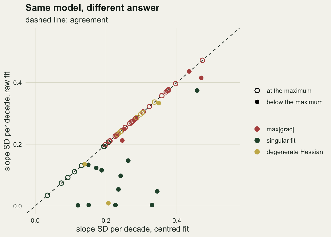
Whether the optimisers start independently matters, because since lme4 1.1-38 allFit() by default starts every optimiser from the estimates of the fit it was given (start_from_mle = TRUE); the allFit() calls above switch this off where the argument exists. The chunk below imitates the new default on all the raw fits that ended below the maximum: each of the five optimisers is restarted from the fit’s own estimates with update(fit, start = ...), which is what allFit() does internally.
max_arg <- c(bobyqa = "maxfun", Nelder_Mead = "maxfun", nlminbwrap = "eval.max", nloptwrap = "maxeval")
from_mle <- function(fit, d) {
  pars <- getME(fit, c("theta", "fixef"))
  vapply(seq_len(nrow(opt_tab)), function(j) {
    op <- opt_tab[j, "optimizer"]; oc <- list(); oc[[max_arg[[op]]]] <- 1e5
    if (op == "nloptwrap") oc$algorithm <- opt_tab[j, "method"]
    f <- tryCatch(quiet(update(fit, start = pars, data = d,
                               control = glmerControl(optimizer = op, optCtrl = oc))),
                  error = function(e) NULL)
    if (is.null(f)) NA_real_ else as.numeric(logLik(f)) }, 0)
}
ms <- do.call(rbind, lapply(which(sl$wrong), function(i) {
  ll <- from_mle(slope_raw_fits[[i]], slope_surveys[[i]])
  data.frame(survey = i, n_run = sum(!is.na(ll)), spread = diff(range(ll, na.rm = TRUE)),
             n_reach = sum(sl$ll_ref[i] - ll < 0.01, na.rm = TRUE),
             sing = sl$type_raw[i] == "singular fit")
}))
ms_seen  <- sum(ms$spread > 0.01)
ms_none  <- sum(ms$n_reach == 0)
ms_stuck <- ms$n_reach == 0 & ms$spread < 0.01
Started from their own wrong estimates, the five optimisers still spread by more than 0.01 log-likelihood units in 18 of the 23 wrong fits, and at least one of them reaches the maximum in 14. In 9 none of the five gets there, and in 5 all five agree to within 0.01 units on the wrong point, every one of them a singular fit: started on the boundary, they stay on it. (In 2 of the 23, one or more restarts stopped with an error and are left out.) By the usual reading that agreement would pass the fit. Independent starts are what make allFit() a test of the maximum; started from the fit’s own estimates it can pass a fit that is wrong.
What to do with the warning
Centre calendar years, distances and elevations on a value inside the data before fitting, and put them in units in which one step is a sensible change: decades, kilometres, hundreds of metres. Schielzeth 2010 recommends centring and scaling inputs so that coefficients can be interpreted; here it also decided whether the standard error was right and whether a random-slope fit reached its maximum. Centring did most of the work in these surveys; rescaling without centring left the warning in place, though the standard errors survived it.
When the warning appears anyway, the cross-check is a refit, not a second look at the gradient. Refit with the predictors centred and rescaled, and compare the log-likelihood, the estimates converted back to the original units, and the standard errors. If all three agree and the refit is quiet, report the refit, which is the same model. If the log-likelihoods differ, the fit with the higher one is the maximum, whatever messages either carries. Run allFit() as well when the model has several variance parameters, with independent starts (in lme4 1.1-38 and later, allFit(..., start_from_mle = FALSE): the new default starts every optimiser from the original fit and can leave all of them on the same boundary point), because disagreement between optimisers is the evidence that the search is in trouble; but do not read agreement between them as a clean bill for the standard errors. A quicker check of the standard errors alone is vcov(fit, use.hessian = FALSE): if it disagrees with the default standard errors, refit. It does not test the maximum. In the random-slope surveys it differed from the default standard error by more than ten per cent in 3 of the 23 raw fits below the maximum.
lme4_ver <- packageVersion("lme4")
newer <- lme4_ver >= "1.1.38"
if (newer) stopifnot("autoscale" %in% names(formals(glmerControl)),
                     glmerControl()$checkConv$check.conv.nobsmax == 1e4,
                     isTRUE(formals(allFit)$start_from_mle))
# the construction-time scale message, triggered on a column with SD above 1000
scale_msg <- tryCatch(getFromNamespace("checkScaleX", "lme4")(cbind(x = c(1, 2e4, 3, 5e4)), kind = "warning"),
                      warning = conditionMessage)
stopifnot(grepl("very different scales: consider rescaling", scale_msg, fixed = TRUE),
          grepl("autoscale = TRUE", scale_msg, fixed = TRUE) == newer)
Three changes in newer lme4 bear on this. From version 1.1-38 the finite-difference derivatives are not computed at all for data with 10000 or more observations, for models with many parameters and for singular fits, so such a fit prints no max|grad| warning and its standard errors come from the fixed-effect model matrix instead of a finite-difference Hessian. Version 1.1-38 also added glmerControl(autoscale = TRUE), which centres and scales the predictors internally and reports the results on the original scale, and the scale message now mentions it. And from the same version allFit() starts every optimiser from the original fit unless start_from_mle = FALSE is given, which the code on this page does wherever the argument exists. This page was run with lme4 2.0.1, which has all three.
What to report
Say in which units each predictor entered the model, and whether it was centred and on what value. A reader cannot judge a max|grad| warning, or its absence, without that.
Report the convergence messages the final fit carried, from the fit object, not a paraphrase. If the reported fit was refitted after a warning, say what was compared and by how much the two fits differed in log-likelihood, estimate and standard error.
For a random slope, report the slope standard deviation from a fit in centred units. A near-zero slope variance from a raw calendar year fit is not evidence that the trends are the same in every wood.
Honest limits
Everything here is one design: Poisson counts, fifteen to two hundred and forty woods, twenty consecutive years, one wood-level covariate and a random intercept or a random intercept and slope. The damage comes from a covariate far from zero, and calendar years are the commonest case in monitoring data, but other offsets (elevation in metres above sea level, day of year in late summer) will do it to different degrees, and binomial and negative binomial models, crossed random effects and models with many variance parameters were not simulated.
None of the twenty surveys at the largest size had a wrong standard error, and a zero out of twenty is still compatible with a true share of up to 17 per cent (the exact 95 per cent upper bound). The rates depend on the linear algebra library and on the optimiser code of the machine that runs the page, so the numbers printed here can move on another machine; the stored-message rates and the comparisons are computed, not assumed.
The reference throughout is the fit in centred and rescaled units, not a proven maximum. It was never beaten by any other coding or optimiser here, and in the worked example its Hessian standard error of 0.0510 sits close to the one from the fixed-effect model matrix, 0.0512. The claim that the raw standard errors are too small does not rest on the reference alone: the coverage check against the true decline, in the section on standard errors, points the same way. The standard errors compared are Wald standard errors. Profile likelihood intervals were not examined, and they do not use the finite-difference Hessian, so they may behave differently.
Genuine failures of other kinds, on predictors that are already centred and scaled, were not constructed here. A quiet fit in centred units says that this particular problem is gone, not that the model is identified.
References
Bates D, Maechler M, Bolker B, Walker S 2015 Journal of Statistical Software 67(1) (10.18637/jss.v067.i01)
Schielzeth H 2010 Methods in Ecology and Evolution 1(2):103-113 (10.1111/j.2041-210X.2010.00012.x)
Nelder JA, Mead R 1965 The Computer Journal 7(4):308-313 (10.1093/comjnl/7.4.308)