library(ggplot2)
library(lme4)
library(nlme)

te_paper  <- "#f5f4ee"
te_ink    <- "#16241d"
te_body   <- "#2c3a31"
te_forest <- "#275139"
te_rust   <- "#b5534e"
te_gold   <- "#c9b458"
te_line   <- "#dad9ca"

theme_datasheet <- function() {
  theme_minimal(base_size = 12) +
    theme(plot.background  = element_rect(fill = te_paper, colour = NA),
          panel.background = element_rect(fill = te_paper, colour = NA),
          panel.grid.major = element_line(colour = te_line, linewidth = 0.3),
          panel.grid.minor = element_blank(),
          text             = element_text(colour = te_body),
          plot.title       = element_text(colour = te_ink, face = "bold"),
          plot.subtitle    = element_text(colour = te_body),
          axis.text        = element_text(colour = te_body),
          strip.text       = element_text(colour = te_ink))
}AIC on REML fits: when units choose the model
R
mixed models
model selection
AIC
lme4
nlme
simulation
ecology tutorial
lme4 ranks REML fits with different fixed effects without a word. Measuring in R how writing elevation in metres or kilometres then decides the chosen model.
Twenty grassland sites climb a hillside from 60 to 390 m above sea level, and each has been cut and weighed in the same week of June for six years. The response is above-ground biomass in tonnes of dry matter per hectare, the question is whether yield falls with elevation, and the site is a random intercept because the six harvests from one meadow share its soil and its management. The model is fitted with lmer(), which estimates by restricted maximum likelihood (REML) unless told otherwise, and the comparison is the one every model selection tutorial teaches: fit the model with elevation and the model without it, and keep the one with the lower AIC.
A colleague reruns the script with elevation converted to kilometres, because the axis labels look tidier. In most datasets of this design that is enough to change the verdict, although nothing about the data, the model or the fit has changed except the numbers printed in one column. That is the subject of this post.
The rule behind it is old and it is stated on this site already. AIC with missing values: the silent row drop has one sentence near the end of its honest limits saying that fits with different fixed-effect structures estimated by REML are not comparable by AIC, for a reason about what the likelihood is a likelihood of; it does not measure anything about it. The nlme package that goes with Pinheiro and Bates (2000) prints the rule as a warning, shown below, and the ecological protocol of Zuur and colleagues (2009) is built around it: compare random structures with REML, compare fixed effects with maximum likelihood (ML). This post is a demonstration of that known rule, not a new result. What it adds is the size of the error and its direction, both of which are set by the units of the covariate, and how often that decides the model.
Model selection with AIC in R for ecology covers what AIC is and names one unit trap already: with a log-transformed response the Jacobian of the transformation depends on the units of the response. The trap here is a second one, and it sits in the REML log likelihood as lme4 and nlme compute it. Two of the nlme posts that compare REML fits by AIC, Modelling non-constant variance with nlme and Random slopes in mixed models with nlme, both keep the fixed part identical across the models they compare, which is the case where the comparison is legitimate; that case is measured below as well: its AIC differences do not move with the unit.
Twenty meadows and three codings of one covariate
The design is fixed and balanced: twenty sites evenly spaced in elevation, six years at each. Biomass has a mean of 3 t/ha, a site standard deviation of 0.4 t/ha and a residual standard deviation of 0.5 t/ha. Under the null elevation does nothing; under the alternative biomass falls by 0.2 t/ha per 100 m. Year appears in the data frame but not in the generating model, which will matter later. All of these constants were fixed before anything was run.
n_site <- 20; n_year <- 6
elev_site <- seq(60, 390, length.out = n_site)       # metres above sea level
mu0 <- 3.0; sd_site <- 0.4; sd_res <- 0.5             # t/ha
slope_alt <- -0.2                                     # t/ha per 100 m

meadows <- data.frame(site = factor(rep(seq_len(n_site), each = n_year)),
                      year = factor(rep(seq_len(n_year), n_site)))
meadows$elev_m  <- elev_site[as.integer(meadows$site)]
meadows$elev_km <- meadows$elev_m / 1000
meadows$elev_z  <- (meadows$elev_m - mean(elev_site)) / sd(elev_site)
elev_sd <- sd(elev_site)

draw_biomass <- function(slope_100m) {
  mu0 + slope_100m * (meadows$elev_m - mean(elev_site)) / 100 +
    rnorm(n_site, 0, sd_site)[meadows$site] + rnorm(nrow(meadows), 0, sd_res)
}

set.seed(4100)
meadows$biomass <- draw_biomass(0)

fit_null <- lmer(biomass ~ 1 + (1 | site), data = meadows)
fit_m    <- lmer(biomass ~ elev_m  + (1 | site), data = meadows)
fit_km   <- lmer(biomass ~ elev_km + (1 | site), data = meadows)
fit_z    <- lmer(biomass ~ elev_z  + (1 | site), data = meadows)
stopifnot(isTRUE(formals(lmer)$REML), isREML(fit_m))   # lmer default is REML

AIC(fit_null, fit_m, fit_km, fit_z)
df AIC
fit_null 3 206.0908
fit_m 4 220.1025
fit_km 4 206.2870
fit_z 4 210.8379daic_m <- AIC(fit_m) - AIC(fit_null)
daic_km <- AIC(fit_km) - AIC(fit_null)
daic_z <- AIC(fit_z) - AIC(fit_null)
gap_m_km <- AIC(fit_m) - AIC(fit_km)
same_theta <- max(abs(c(getME(fit_m, "theta") - getME(fit_km, "theta"),
getME(fit_m, "theta") - getME(fit_z, "theta"))))
same_sigma <- max(abs(sigma(fit_m) - c(sigma(fit_km), sigma(fit_z))))
same_fitted <- max(abs(c(fitted(fit_m) - fitted(fit_km), fitted(fit_m) - fitted(fit_z))))
slope_err <- abs(fixef(fit_km)[["elev_km"]] / 1000 - fixef(fit_m)[["elev_m"]])
daic_mile <- daic_m - 2 * log(1609.344) # elevation in statute milesThis dataset was drawn under the null. Against the model without elevation, the elevation model has an AIC difference of +14.01 with elevation in metres, +0.20 in kilometres and +4.75 as a standardised score, where a negative difference would mean that elevation enters. In this dataset all three codings keep it out, but by margins that differ only because of the unit: 14.0 units in metres, 0.20 in kilometres. Written in statute miles, the same fit gives -0.76 and elevation would be in the model.
The elevation fits are one model. Their variance estimates and fitted values agree to within floating-point rounding, and the slope per kilometre equals the slope per metre times 1000 to the same precision. Yet the AIC of the metre fit minus the AIC of the kilometre fit is 13.8155. lmer() returned all of this without a warning.
Where the shift comes from
For a linear mixed model with fixed-effect design matrix X (n rows, p columns), marginal covariance V and generalised least squares residual r, the restricted likelihood of Patterson and Thompson (1971), reviewed with the other likelihood approaches by Harville (1977), is computed by lme4 (Bates and colleagues 2015) and nlme as
l_R = -0.5 * [ (n - p) log(2 pi) + log det(V) + log det(X' V^-1 X) + r' V^-1 r ]Only one term involves the columns of X other than through r. Rescale the elevation column by a factor c, from metres to kilometres say, and X becomes X D, with D diagonal holding a one for the intercept and 1 / c for elevation. The determinant term then drops by 2 log(c), while V, r and therefore the maximising variance parameters do not change. l_R rises by exactly log(c) at every value of the variance parameters, and AIC falls by 2 log(c). The null model has no elevation column and does not move. For c = 1000 that is 2 log(1000), and centring the covariate changes nothing because it multiplies X by a triangular matrix with unit determinant; only the scale enters.
This is not a property of lme4: nlme computes the same quantity, as shown further down. It is a property of the REML log likelihood in this form, which leaves out a term +0.5 log det(X' X). That term is constant while X is fixed, so it never matters for estimation, and dropping it is common. Across models with different X it is not constant, and it is exactly what moves with the unit of elevation. Put it back and the result is the density of n - p orthonormal error contrasts, the combinations of the data that the fixed effects cannot reach, and that density does not depend on the unit of elevation. The comparison is still not legitimate. Two models with different X remove different things, so their REML likelihoods are densities of different data, and the unit of the response still moves them: multiplying the response by a lowers l_R, with or without the extra term, by (n - p) log(a), which is a real Jacobian, and a model with one more fixed column loses one log(a) less. Converting biomass from t/ha to grams per square metre (a factor of 100) therefore lowers the AIC gap by 2 log(100), in the same direction as the change from metres to kilometres: both make the slope’s numbers larger. The chunk below writes l_R out by hand at the lme4 estimates and compares it with logLik(), builds the contrast density directly from an orthonormal basis, and refits with biomass in grams.
reml_by_hand <- function(fit) {
  X <- getME(fit, "X"); Z <- as.matrix(getME(fit, "Z"))
  lam <- as.matrix(getME(fit, "Lambda")); y <- getME(fit, "y")
  V <- sigma(fit)^2 * (diag(nrow(X)) + Z %*% lam %*% t(lam) %*% t(Z))
  Vi <- solve(V); XtViX <- t(X) %*% Vi %*% X
  r <- y - X %*% solve(XtViX, t(X) %*% Vi %*% y)
  n <- nrow(X); p <- ncol(X)
  as.numeric(-0.5 * ((n - p) * log(2 * pi) + determinant(V)$modulus +
                     determinant(XtViX)$modulus + t(r) %*% Vi %*% r))
}
hand_gap <- max(abs(sapply(list(fit_null, fit_m, fit_km, fit_z), reml_by_hand) -
                    sapply(list(fit_null, fit_m, fit_km, fit_z), function(f) as.numeric(logLik(f)))))
shift_err_km <- abs(gap_m_km - 2 * log(1000))
shift_err_z  <- abs((AIC(fit_m) - AIC(fit_z)) - 2 * log(elev_sd))
c(hand_gap = hand_gap, shift_err_km = shift_err_km, shift_err_z = shift_err_z)
hand_gap shift_err_km shift_err_z
1.136868e-13 5.684342e-14 5.506706e-14 meadows$biomass_g <- 100 * meadows$biomass # t/ha to g per square metre
fit_g1 <- lmer(biomass_g ~ elev_m + (1 | site), data = meadows)
fit_g0 <- lmer(biomass_g ~ 1 + (1 | site), data = meadows)
daic_m_g <- AIC(fit_g1) - AIC(fit_g0)
resp_err <- abs((daic_m_g - daic_m) + 2 * log(100))
contrast_by_hand <- function(fit) { # density of n - p orthonormal error contrasts
X <- getME(fit, "X"); Z <- as.matrix(getME(fit, "Z"))
lam <- as.matrix(getME(fit, "Lambda")); y <- getME(fit, "y")
V <- sigma(fit)^2 * (diag(nrow(X)) + Z %*% lam %*% t(lam) %*% t(Z))
K <- qr.Q(qr(X), complete = TRUE)[, -seq_len(ncol(X)), drop = FALSE] # K'X = 0, K'K = I
w <- crossprod(K, y); S <- crossprod(K, V %*% K)
as.numeric(-0.5 * (length(w) * log(2 * pi) + determinant(S)$modulus + crossprod(w, solve(S, w))))
}
half_logdet_xx <- function(fit) 0.5 * as.numeric(determinant(crossprod(getME(fit, "X")))$modulus)
fits_4 <- list(fit_null, fit_m, fit_km, fit_z)
contrast_ll <- sapply(fits_4, contrast_by_hand)
contrast_err <- max(abs(contrast_ll - sapply(fits_4, function(f) as.numeric(logLik(f))) -
sapply(fits_4, half_logdet_xx)))
contrast_daic <- -2 * (contrast_ll[2:4] - contrast_ll[1]) + 2 # metres, km, SD score
contrast_gap <- diff(range(contrast_daic))
contrast_resp_err <- abs((-2 * (contrast_by_hand(fit_g1) - contrast_by_hand(fit_g0)) + 2) -
contrast_daic[1] + 2 * log(100))
stopifnot(hand_gap < 1e-6, contrast_err < 1e-6, contrast_gap < 1e-6, contrast_resp_err < 1e-6)The hand formula and logLik() agree to within floating-point rounding across the four fits (hand_gap in the output above), so lme4 reports exactly this quantity for a REML fit. The metre-minus-kilometre gap of 13.8155 is 2 log(1000) = 13.8155 to within the same rounding (shift_err_km), and the standardised score, which divides by the standard deviation of the site elevations (102.8 m), sits 9.2647 below the metre fit, which is twice the log of that standard deviation, again to within rounding (shift_err_z). The shift is reproduced, not discovered: it is arithmetic, and the check is that the software follows it to machine precision. The contrast density built from an orthonormal basis equals logLik() plus 0.5 log det(X' X) to within floating-point rounding across the same four fits, and on that scale the elevation model has an AIC difference of +0.011 against the null in metres, in kilometres and as a standardised score alike (the three are equal up to rounding). With biomass in grams per square metre and elevation in metres the lme4 difference becomes +4.80, which is the t/ha value minus 2 log(100) up to rounding, and the contrast-density difference moves by the same 2 log(100), also up to rounding. What sets the shift in lme4’s AIC is the unit of the slope, response units per covariate unit. The rest of the post keeps biomass in t/ha and varies only the elevation unit.
unit_tab <- data.frame(unit  = c("1 m", "10 m", "100 m", "1 km", "10 km", "1 SD", "1 mile"),
                       size_m = c(1, 10, 100, 1000, 10000, elev_sd, 1609.344),
                       lab_pos = c("above", "above", "above", "right", "above", "left", "left"))
aic_null_r <- AIC(fit_null)
fit_null_ml <- lmer(biomass ~ 1 + (1 | site), data = meadows, REML = FALSE)
unit_tab$daic_reml <- NA; unit_tab$daic_ml <- NA
for (i in seq_len(nrow(unit_tab))) {
  meadows$elev_u <- (meadows$elev_m - mean(elev_site)) / unit_tab$size_m[i]
  unit_tab$daic_reml[i] <- AIC(lmer(biomass ~ elev_u + (1 | site), data = meadows)) - aic_null_r
  unit_tab$daic_ml[i]   <- AIC(lmer(biomass ~ elev_u + (1 | site), data = meadows,
                                    REML = FALSE)) - AIC(fit_null_ml)
}
line_tab <- data.frame(size_m = 10^seq(-0.3, 4.3, length.out = 200))
line_tab$daic <- daic_m - 2 * log(line_tab$size_m)
sweep_err <- max(abs(unit_tab$daic_reml - (daic_m - 2 * log(unit_tab$size_m))))
ml_spread <- diff(range(unit_tab$daic_ml))
break_even <- exp(daic_m / 2)       # unit size in metres at which the REML difference is zero
lp <- unit_tab$lab_pos; unit_tab$lab_h <- c(above = 0.5, left = 1, right = 0)[lp]
unit_tab$lab_x <- unit_tab$size_m * c(above = 1, left = 0.87, right = 1.15)[lp]
unit_tab$lab_y <- unit_tab$daic_reml + c(above = 1.6, left = -1.2, right = 1.0)[lp]ggplot(unit_tab, aes(size_m, daic_reml)) +
annotate("rect", xmin = 0.5, xmax = 2e4, ymin = -Inf, ymax = 0,
fill = te_gold, alpha = 0.15) +
geom_hline(yintercept = 0, colour = te_body, linewidth = 0.4) +
geom_hline(yintercept = unit_tab$daic_ml[1], colour = te_rust,
linetype = "dashed", linewidth = 0.8) +
geom_line(data = line_tab, aes(size_m, daic), colour = te_forest, linewidth = 0.9) +
geom_point(size = 3, colour = te_forest) +
geom_text(aes(lab_x, lab_y, label = unit, hjust = lab_h), colour = te_ink, size = 3.6) +
scale_x_log10(breaks = c(1, 10, 100, 1000, 10000),
labels = c("1 m", "10 m", "100 m", "1 km", "10 km")) +
annotate("text", x = 1.2, y = unit_tab$daic_ml[1] - 1.3, hjust = 0,
label = "ML difference, same in every unit", colour = te_rust, size = 3.6) +
annotate("text", x = 1.2, y = -7.5, hjust = 0,
label = "below zero: elevation enters", colour = te_body, size = 3.6) +
labs(x = "unit of elevation (log scale)", y = "AIC with elevation minus AIC without",
title = "The unit decides the sign of the REML comparison",
subtitle = "green: REML fits, rust dashed: ML fits") +
theme_datasheet()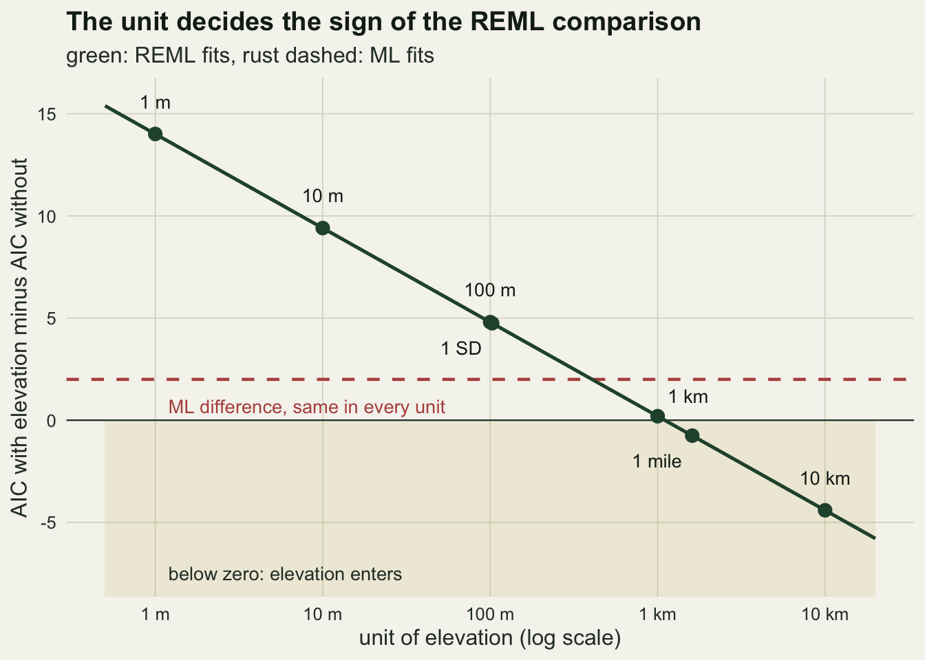
Across the 7 codings the separate fits sit on the line dAIC_m - 2 log(u), where dAIC_m is the difference in metres and u the unit in metres, to within floating-point rounding. The ML differences for the same codings are equal up to rounding: under ML the comparison is +2.00 whatever the unit. For this dataset the REML comparison changes sign at a unit of 1103 m: any coarser unit lets elevation in, any finer one keeps it out.
With the same fixed effects the shift cancels
The shift is a property of X alone, so two REML fits with the same fixed effects receive the same shift and their difference is untouched. That is why the nlme posts linked above are right to compare variance structures under REML. Here the check is a random intercept for year, which is not in the generating model: both candidates contain elevation, one adds (1 | year), a crossed term of the kind explained in Nested and crossed random effects in lme4. It is run on a verification set of fresh null datasets, fitting every coding separately rather than trusting the algebra.
n_ver <- 100                                   # fixed before running
form_of <- function(v, yr = FALSE) reformulate(c(v, "(1 | site)", if (yr) "(1 | year)"), "biomass")
cod <- c(m = "elev_m", km = "elev_km", z = "elev_z")
templ <- c(list(r0 = lmer(form_of("1"), data = meadows)),
  setNames(lapply(cod, function(v) lmer(form_of(v), data = meadows)), paste0("r_", names(cod))),
  setNames(lapply(cod, function(v) lmer(form_of(v, TRUE), data = meadows)), paste0("ry_", names(cod))),
  list(m0 = lmer(form_of("1"), data = meadows, REML = FALSE)),
  setNames(lapply(cod[1:2], function(v) lmer(form_of(v), data = meadows, REML = FALSE)),
           c("m_m", "m_km")))
warn_log <- character(0)                       # lme4 convergence warnings, logged by model
refit_quiet <- function(ft, yb, nm = "rate") withCallingHandlers(suppressMessages(refit(ft, yb)),
  warning = function(w) { warn_log <<- c(warn_log, nm); invokeRestart("muffleWarning") })
set.seed(4103)
ver <- t(replicate(n_ver, {
  yb <- draw_biomass(0)
  a <- vapply(names(templ), function(nm) AIC(refit_quiet(templ[[nm]], yb, nm)), 0)
  c(fixed_m = a[["r_m"]] - a[["r0"]], fixed_km = a[["r_km"]] - a[["r0"]],
    fixed_z = a[["r_z"]] - a[["r0"]],
    year_m = a[["ry_m"]] - a[["r_m"]], year_km = a[["ry_km"]] - a[["r_km"]],
    year_z = a[["ry_z"]] - a[["r_z"]],
    ml_m = a[["m_m"]] - a[["m0"]], ml_km = a[["m_km"]] - a[["m0"]])
}))
ver_fixed_err <- max(abs(ver[, "fixed_m"] - ver[, "fixed_km"] - 2 * log(1000)))
ver_year_diff <- max(abs(c(ver[, "year_m"] - ver[, "year_km"], ver[, "year_m"] - ver[, "year_z"])))
ver_ml_diff   <- max(abs(ver[, "ml_m"] - ver[, "ml_km"]))
year_pick     <- mean(ver[, "year_m"] < 0)
year_pick_agree <- all((ver[, "year_m"] < 0) == (ver[, "year_km"] < 0) &
                       (ver[, "year_m"] < 0) == (ver[, "year_z"] < 0))
n_flip_ver <- sum((ver[, "fixed_m"] < 0) != (ver[, "fixed_km"] < 0))
n_warn_ver <- length(warn_log)
warn_year_only <- all(startsWith(warn_log, "ry_"))   # which models warned
Over 100 datasets the elevation comparison in metres and in kilometres differs by 2 log(1000) to within floating-point rounding every time, and the verdict flips between the two codings in 65 of them. The year comparison, with elevation in both models, gives the same AIC difference in all three codings to within \(2.6 \times 10^{-8}\), and the year term is chosen in the same datasets whichever coding is used (every dataset agrees; the term is picked in 3 per cent of these null datasets, the same number in all three). The ML comparison of elevation is the same in metres and in kilometres up to rounding. Of the 1000 refits, 3 raised the lme4 convergence warning, all of them year models; they are kept, and they obey the same equalities.
same_tab <- rbind(
  data.frame(panel = "REML, elevation vs none", x = ver[, "fixed_m"], y = ver[, "fixed_km"]),
  data.frame(panel = "REML, year term", x = ver[, "year_m"], y = ver[, "year_km"]),
  data.frame(panel = "ML, elevation vs none", x = ver[, "ml_m"], y = ver[, "ml_km"]))
same_tab$panel <- factor(same_tab$panel, levels = unique(same_tab$panel))
ggplot(same_tab, aes(x, y)) +
  geom_abline(slope = 1, intercept = 0, colour = te_body, linetype = "dashed", linewidth = 0.5) +
  geom_hline(yintercept = 0, colour = te_line, linewidth = 0.6) +
  geom_vline(xintercept = 0, colour = te_line, linewidth = 0.6) +
  geom_point(colour = te_forest, alpha = 0.6, size = 1.8) +
  facet_wrap(~ panel, scales = "free") +
  labs(x = "AIC difference, elevation in metres",
       y = "AIC difference, elevation in km",
       title = "Only the REML comparison of fixed effects moves",
       subtitle = sprintf("left panel: every point sits %.1f units below the dashed line",
                         2 * log(1000))) +
  theme_datasheet()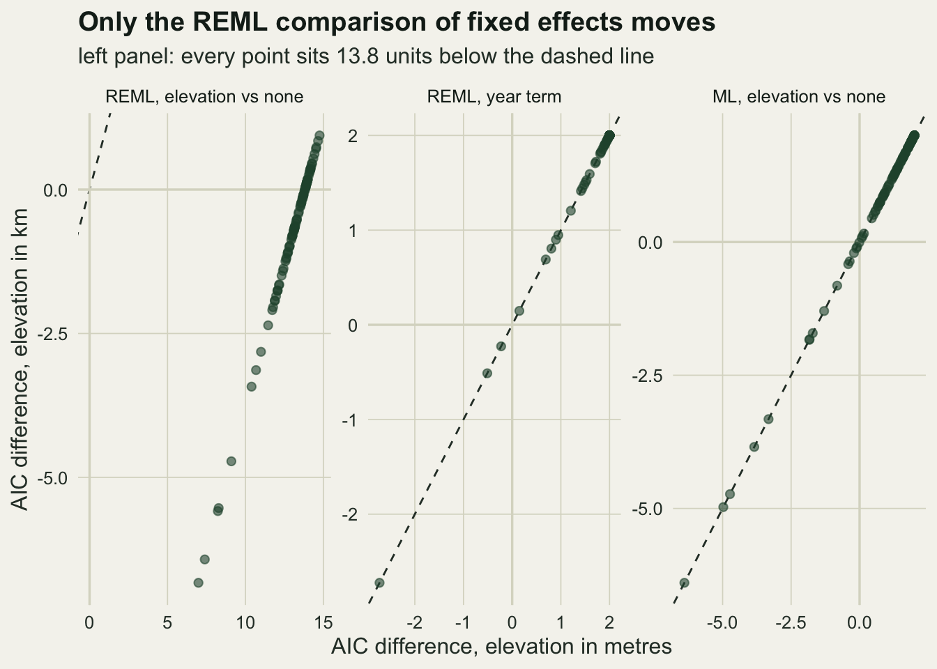
What the REML term measures
The shift has a readable meaning. Hold the variance parameters fixed and l_R is the ML log likelihood profiled over the fixed effects plus (p / 2) log(2 pi) - 0.5 log det(X' V^-1 X). Adding one column changes the last term by minus a half of the log of the information about its coefficient, and that is the log of the coefficient’s standard error. So, at common variance parameters,
dAIC_REML = dAIC_ML - log(2 pi SE^2)where SE is the standard error of the elevation slope from the REML fit, in the units in which it was fitted. A slope that is known precisely in its own units is penalised, and one known vaguely is let in more easily. Converting metres to kilometres multiplies the standard error by 1000, which is the 2 log(1000) again.
In a real fit each model uses its own variance estimates, so the identity is not exact. In this balanced design with a covariate that is constant within a site it can be made exact. The likelihood splits into a within-site part, which is the same for both models, and a part for the twenty site means, which is an ordinary regression of the means on elevation. Working that through, as long as neither fit is singular, the ML difference is 2 - J log(1 + F / (J - 2)) and the REML difference exceeds dAIC_ML - log(2 pi SE^2) by (J - 1) log((J - 1) / (J - 2)) - 1 + log(1 + F / (J - 2)), where J is the number of sites and F the F statistic of the site-means regression. Both claims are checked below on simulated datasets.
The simulation draws 800 datasets under the null and as many under the real decline, and fits each four times: REML and ML, with and without elevation. Warnings from the lme4 convergence check are counted rather than printed.
n_rep <- 800                                   # per scenario, fixed before running
scen_lev <- c("no effect of elevation", "decline of 0.2 t/ha per 100 m")
templ_rate <- templ[c("r0", "r_m", "m0", "m_m")]
warn_log <- character(0)
elev_c <- elev_site - mean(elev_site); sxx_m <- sum(elev_c^2)
sim_scenario <- function(slope_100m) t(replicate(n_rep, {
  yb <- draw_biomass(slope_100m)
  f <- lapply(templ_rate, refit_quiet, yb = yb)
  ybar <- as.vector(tapply(yb, meadows$site, mean))
  rss1 <- sum(lm.fit(cbind(1, elev_c), ybar)$residuals^2)
  rss0 <- sum((ybar - mean(ybar))^2)
  c(reml_m = AIC(f$r_m) - AIC(f$r0), ml = AIC(f$m_m) - AIC(f$m0),
    se_m = sqrt(vcov(f$r_m)[2, 2]), f_stat = (rss0 - rss1) / (rss1 / (n_site - 2)),
    singular = isSingular(f$r0) || isSingular(f$r_m) || isSingular(f$m0) || isSingular(f$m_m))
}))
set.seed(4101); sim_null <- sim_scenario(0)
set.seed(4102); sim_alt  <- sim_scenario(slope_alt)
sims <- rbind(sim_null, sim_alt)
n_singular <- sum(sims[, "singular"])

corr_bal <- function(f_stat) (n_site - 1) * log((n_site - 1) / (n_site - 2)) - 1 +
                             log(1 + f_stat / (n_site - 2))
gap_general <- sims[, "reml_m"] - (sims[, "ml"] - log(2 * pi * sims[, "se_m"]^2))
ok <- sims[, "singular"] == 0
exact_err_reml <- max(abs(gap_general[ok] - corr_bal(sims[ok, "f_stat"])))
exact_err_ml <- max(abs(sims[ok, "ml"] - (2 - n_site * log(1 + sims[ok, "f_stat"] / (n_site - 2)))))
gap_q <- quantile(gap_general, c(0.5, 0.9, 1))
corr_min <- corr_bal(0)
Across the 1600 datasets the general identity leaves a gap: the REML difference exceeds dAIC_ML - log(2 pi SE^2) by a median of 0.117 AIC units, a 90th percentile of 0.425 and a maximum of 1.226, all small against the 13.8 units between metres and kilometres. The balanced-design version accounts for that gap to within \(4.4 \times 10^{-4}\), and the ML formula holds to within \(2.7 \times 10^{-6}\), on the 1600 datasets in which no fit was singular (0 had a singular fit). The gap is never below 0.0273, its value at an F of zero. 2 of the 6400 refits raised the lme4 convergence warning; their AIC differences obey the same identities.
How often the unit decides
A single dataset shows the mechanism; the rate at which it changes a decision needs many. For each dataset the REML difference in any unit is the difference in metres minus 2 log(u), verified above to machine precision, so every dataset has a break-even unit u* = exp(dAIC_m / 2) at which it changes its verdict, and elevation is chosen for every unit coarser than u*. The share of datasets that choose elevation, as a function of the unit, is the empirical distribution function of u*.
The closed forms of the previous section also give these rates without simulation. The residual sum of squares of the site-means regression is the variance of a site mean times a chi-squared variate on J - 2 degrees of freedom, and the extra sum of squares for elevation is an independent chi-squared on one degree of freedom, noncentral under the decline. The ML rate is then a noncentral F probability, and the REML rate a one-dimensional integral over the first chi-squared. The simulation is a check on those formulas, not a separate finding.
shift_of <- c(m = 0, km = -2 * log(1000), z = -2 * log(elev_sd))
pick <- function(sim) c(sapply(shift_of, function(s) mean(sim[, "reml_m"] + s < 0)),
                        ml = mean(sim[, "ml"] < 0))
rate_null <- pick(sim_null); rate_alt <- pick(sim_alt)
mcse <- function(p) sqrt(p * (1 - p) / n_rep)
mcse_max <- mcse(0.5)
n_pick_null_m <- sum(sim_null[, "reml_m"] < 0)

tau2 <- sd_site^2 + sd_res^2 / n_year               # variance of a site mean
lam_alt <- (slope_alt / 100)^2 * sxx_m / tau2       # noncentrality under the decline
k_const <- (n_site - 1) * log(n_site - 1) - (n_site - 2) * log(n_site - 2) + 1
rate_reml_cf <- function(u, lam) integrate(function(q1) {
  g <- k_const + log(sxx_m / u^2 / (2 * pi)) - log(tau2 * q1)
  thr <- ifelse(g > 0, q1 * (exp(g / (n_site - 1)) - 1), 0)
  dchisq(q1, n_site - 2) * pchisq(thr, 1, ncp = lam, lower.tail = FALSE)
}, 0, Inf)$value
ml_crit <- (n_site - 2) * (exp(2 / n_site) - 1)
cf_null <- c(sapply(c(1, 1000, elev_sd), rate_reml_cf, lam = 0),
             pf(ml_crit, 1, n_site - 2, lower.tail = FALSE))
cf_alt  <- c(sapply(c(1, 1000, elev_sd), rate_reml_cf, lam = lam_alt),
             pf(ml_crit, 1, n_site - 2, ncp = lam_alt, lower.tail = FALSE))
z_dev <- abs(c(rate_null, rate_alt) - c(cf_null, cf_alt)) /
         pmax(mcse(c(cf_null, cf_alt)), 1 / n_rep)
ml_asym <- pchisq(2, df = 1, lower.tail = FALSE)   # large-sample P(LR > 2)
ubreak_null <- exp(sim_null[, "reml_m"] / 2); ubreak_alt <- exp(sim_alt[, "reml_m"] / 2)
q_null <- quantile(ubreak_null, c(0.1, 0.5, 0.9))
q_alt  <- quantile(ubreak_alt, c(0.1, 0.5, 0.9))
Under the null, the REML comparison chooses elevation in none of the 800 datasets when it is coded in metres (a share of 0.000; closed form 0.0002), in a share of 0.041 as a standardised score (0.032) and 0.711 in kilometres (0.722). No Monte Carlo standard error of a rate from 800 datasets can exceed 0.018 (its value at a rate of one half), and no simulated rate is more than 1.4 standard errors from its closed form. A covariate with no effect enters the model in 71 per cent of kilometre analyses and in none of the metre analyses.
With a real decline of 0.2 t/ha per 100 m the REML rates are 0.024 in metres, 0.395 standardised and 0.959 in kilometres (closed forms 0.023, 0.412 and 0.954). So in metres the REML comparison misses a real effect in all but 2 per cent of datasets, and in kilometres it admits a null one in 71 per cent.
These rates belong to this design and these units. They are illustrations of the 2 log(c) shift, not general rates: a response in grams per square metre or a gradient in hundreds of metres would put the three codings at different points on the same curves.
u_grid <- 10^seq(-0.3, 4.3, length.out = 300)
u_cf <- 10^seq(-0.3, 4.3, length.out = 40)
curve_tab <- rbind(
  data.frame(scen = scen_lev[1], u = u_grid, rate = ecdf(ubreak_null)(u_grid)),
  data.frame(scen = scen_lev[2], u = u_grid, rate = ecdf(ubreak_alt)(u_grid)))
cf_tab <- rbind(
  data.frame(scen = scen_lev[1], u = u_cf, rate = sapply(u_cf, rate_reml_cf, lam = 0)),
  data.frame(scen = scen_lev[2], u = u_cf, rate = sapply(u_cf, rate_reml_cf, lam = lam_alt)))
mark_tab <- data.frame(scen = rep(scen_lev, each = 3),
                       u = rep(c(1, elev_sd, 1000), 2),
                       rate = c(rate_null[c("m", "z", "km")], rate_alt[c("m", "z", "km")]),
                       lab = rep(c("metres", "SD score", "km"), 2))
mark_tab$lab_pos <- c("above", "left", "right", "above", "left", "right")
mark_tab$lab_x <- mark_tab$u * c(above = 1, left = 0.8, right = 1.2)[mark_tab$lab_pos]
mark_tab$lab_y <- mark_tab$rate + c(above = 0.07, left = 0.05, right = -0.06)[mark_tab$lab_pos]
mark_tab$lab_h <- c(above = 0.5, left = 1, right = 0)[mark_tab$lab_pos]
ml_tab <- data.frame(scen = scen_lev, rate = c(rate_null["ml"], rate_alt["ml"]))
for (tb in c("curve_tab", "cf_tab", "mark_tab", "ml_tab"))
  assign(tb, transform(get(tb), scen = factor(scen, levels = scen_lev)))
ggplot(curve_tab, aes(u, rate)) +
  geom_hline(data = ml_tab, aes(yintercept = rate), colour = te_rust,
             linetype = "dashed", linewidth = 0.8) +
  geom_line(colour = te_forest, linewidth = 1.4) +
  geom_line(data = cf_tab, colour = te_ink, linetype = "dotted", linewidth = 0.7) +
  geom_point(data = mark_tab, colour = te_ink, size = 2.6) +
  geom_text(data = mark_tab, aes(x = lab_x, y = lab_y, label = lab, hjust = lab_h),
            colour = te_ink, size = 3.4) +
  facet_wrap(~ scen) +
  scale_x_log10(breaks = c(1, 10, 100, 1000, 10000),
                labels = c("1 m", "10 m", "100 m", "1 km", "10 km")) +
  scale_y_continuous(limits = c(0, 1)) +
  labs(x = "unit of elevation (log scale)", y = "share of datasets keeping elevation",
       title = "The selection rate is a function of the unit",
       subtitle = "points: elevation in metres, as an SD score and in km") +
  theme_datasheet()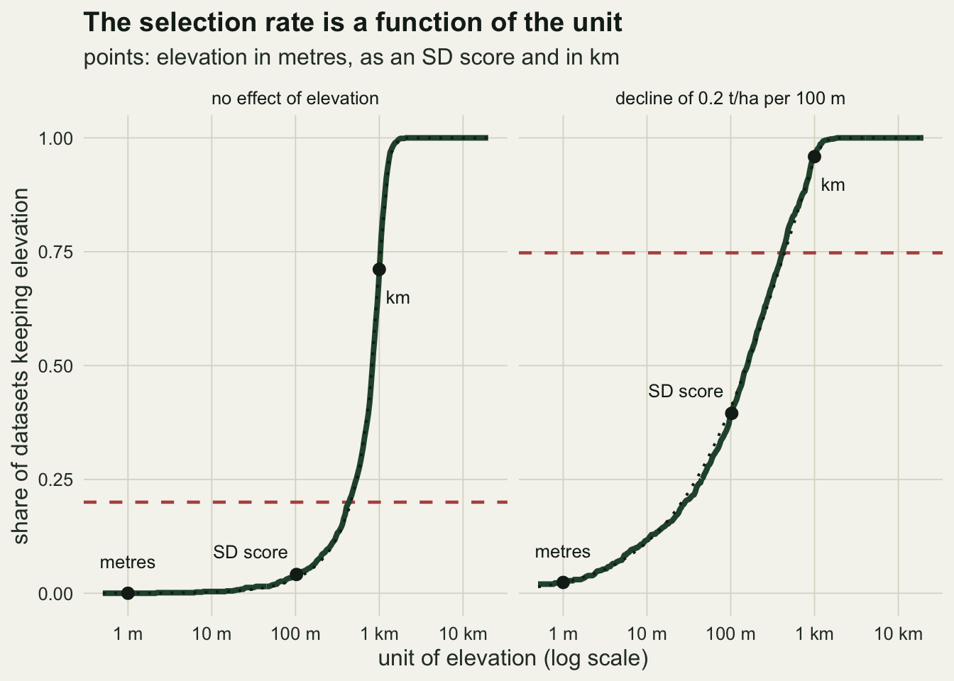
Read as distributions, the curves say where the break-even units lie. Under the null the median break-even unit is 829 m, and the middle 80 per cent of datasets (10th to 90th percentile across the 800) change their verdict somewhere between 253 m and 1193 m. Under the real decline the median is 158 m, with the same percentiles at 8 m and 801 m. Nothing in ecology says what the unit of elevation ought to be, so the REML verdict is set by an arbitrary choice at least as much as by the data.
What lme4 and nlme say
The two packages behave differently, and the difference is where the trap lives. The chunk below captures every warning and message each call raises on the first dataset, and the stopifnot() lines fail the build if a future version behaves differently.
capture_all <- function(expr) {
  conds <- character(0)
  val <- withCallingHandlers(expr,
    warning = function(w) { conds <<- c(conds, paste("warning:", conditionMessage(w)))
                            invokeRestart("muffleWarning") },
    message = function(m) { conds <<- c(conds, paste("message:", trimws(conditionMessage(m))))
                            invokeRestart("muffleMessage") })
  list(value = val, conds = conds)
}
lme4_aic   <- capture_all(AIC(fit_m, fit_null))
lme4_anova <- capture_all(anova(fit_m, fit_null))
lme4_norefit <- capture_all(anova(fit_m, fit_null, refit = FALSE))
nl_m    <- lme(biomass ~ elev_m,  random = ~ 1 | site, data = meadows)
nl_km   <- lme(biomass ~ elev_km, random = ~ 1 | site, data = meadows)
nl_null <- lme(biomass ~ 1,       random = ~ 1 | site, data = meadows)
nlme_aic    <- capture_all(AIC(nl_m, nl_null))
nlme_anova  <- capture_all(anova(nl_m, nl_null))
nlme_same_p <- capture_all(AIC(nl_m, nl_km))

stopifnot(length(lme4_aic$conds) == 0,
          identical(lme4_anova$conds, "message: refitting model(s) with ML (instead of REML)"),
          length(lme4_norefit$conds) == 0,
          identical(nlme_aic$conds,
                    "warning: models are not all fitted to the same number of observations"),
          identical(nlme_anova$conds,
                    "warning: fitted objects with different fixed effects. REML comparisons are not meaningful."),
          length(nlme_same_p$conds) == 0,
          abs(diff(lme4_norefit$value$AIC) - (AIC(fit_m) - AIC(fit_null))) < 1e-8,
          identical(eval(formals(nlme:::lme.formula)$method)[1], "REML"),
          !("REML" %in% names(formals(glmer))))
anova_ml_err <- max(abs(lme4_anova$value$AIC - c(AIC(fit_null_ml), AIC(update(fit_m, REML = FALSE)))))
nlme_same_gap <- diff(nlme_same_p$value$AIC)
nlme_lme4_ll <- max(abs(c(logLik(nl_m) - logLik(fit_m), logLik(nl_km) - logLik(fit_km),
                           logLik(nl_null) - logLik(fit_null))))
for (nm in c("lme4_aic", "lme4_anova", "lme4_norefit", "nlme_aic", "nlme_anova", "nlme_same_p"))
  cat(sprintf("%-13s %s\n", nm,
              if (length(get(nm)$conds)) paste(get(nm)$conds, collapse = " | ") else "(nothing)"))
lme4_aic (nothing)
lme4_anova message: refitting model(s) with ML (instead of REML)
lme4_norefit (nothing)
nlme_aic warning: models are not all fitted to the same number of observations
nlme_anova warning: fitted objects with different fixed effects. REML comparisons are not meaningful.
nlme_same_p (nothing)AIC() on two lme4 REML fits with different fixed effects prints the table and nothing else. anova() on the same pair does the right thing: it refits both models by ML, says so in a message, and its AIC column equals the ML AICs to within \(1.1 \times 10^{-12}\). With refit = FALSE it compares the REML fits as they are, silently, and returns the same REML gap as AIC() (checked in the chunk). Checked in lme4 2.0-1 here and in the current lme4 source on GitHub (version 2.1-0): logLik() of a REML fit returns l_R, which is minus half of what lme4 prints as the REML criterion, with the full number of observations attached, so AIC() sees nothing to object to, and the message lives in anova().
nlme is not silent. Its anova() warns, in so many words, that REML comparisons of different fixed effects are not meaningful. Its AIC() also warns, but for a different reason: nlme’s logLik() for a REML fit reports n - p observations, and base R’s AIC() objects when the counts differ. That warning is about the number of observations, and it disappears when the two models have the same number of fixed coefficients. Two nlme fits of one model, elevation in metres and in kilometres, go through AIC() without a word and differ by 13.82 units. For these REML fits nlme’s logLik() equals lme4’s to within \(8.5 \times 10^{-14}\): it is the same l_R, without the log det(X' X) term. Both warnings were read here in nlme 3.1-168 and in the current nlme source mirrored on GitHub (version 3.1-171), and the base R warning in the current R source.
So the trap is lme4’s AIC(), and every table built from it by hand: a sapply() over a list of lmer() fits, or a loop that collects AIC() values into a data frame. glmer() has no REML argument and fits by maximum likelihood (approximated), so it cannot fall into this.
The fix is maximum likelihood for the comparison
The rule, as Zuur and colleagues (2009) set it out, is to compare fixed effects with ML fits and to report estimates from the REML fit of the chosen model. In lme4 that is REML = FALSE for the candidate set, or anova(), which does the refit itself. On the first dataset:
ml_null <- update(fit_null, REML = FALSE)
ml_m    <- update(fit_m,  REML = FALSE)
ml_km   <- update(fit_km, REML = FALSE)
AIC(ml_null, ml_m, ml_km)
df AIC
ml_null 3 203.2389
ml_m 4 205.2377
ml_km 4 205.2377ml_gap_one <- AIC(ml_m) - AIC(ml_km)
chosen <- if (AIC(ml_m) < AIC(ml_null)) fit_m else fit_null # REML fit, for the estimatesThe two ML fits with elevation have the same AIC up to floating-point rounding, and the model without elevation is kept, so the estimates to report come from the REML fit of that model. Over the simulations the ML comparison chooses the null covariate in 0.200 of datasets (Monte Carlo standard error 0.014, closed form 0.186) and the real decline in 0.748 (standard error 0.015, closed form 0.734), in every unit.
The null rate is not zero, and it is not meant to be: AIC is not a test. The large-sample rate for one added parameter is the chance that a likelihood ratio statistic on one degree of freedom exceeds two, 0.157. The exact rate for twenty sites is higher, 0.186, because the ML likelihood ratio here is a function of an F statistic on 18 denominator degrees of freedom rather than a chi-squared. The simulated rate sits 1.0 standard errors from the exact value and 3.0 from the large-sample one; the argument for the exact value is the derivation, not that one run. What ML removes is the dependence on the unit, which was what decided the REML comparison.
What to report
State the estimation method of every fit that enters an AIC table. For lmer() the default is REML, so an AIC table of lmer() fits that differ in their fixed effects and does not mention REML = FALSE should be read as unit-dependent until shown otherwise.
For fixed-effect comparisons, report AIC from ML fits, or the anova() table with its refitting message intact, and report coefficients and variance components from the REML refit of the chosen model. For comparisons of random-effect or variance structures with the same fixed effects, REML is the right choice and the units do not matter, as the year check above shows.
If a covariate was rescaled or standardised, say in which units the AIC was computed. Under ML that is a detail; under REML with different fixed effects it is the result.
Honest limits
The design is balanced, Gaussian, with one site-level covariate and one random intercept, and the covariate values are fixed across replicates. The 2 log(c) shift is exact for the REML log likelihood as lme4 and nlme compute it, in any linear mixed model, but the selection rates are properties of this design and these units; a covariate that varies within sites, an unbalanced design or more candidate terms would place the codings at different points on the curves. The rates were not measured for any of those.
The comparison here is always between nested models, one covariate against none. Choosing between two different covariates of the same size, elevation against soil depth, has the same problem under REML with a different shape: the verdict then depends on the ratio of the two units, and it was not simulated.
The closed-form rates rest on the balance of the design, on a covariate that is constant within sites and on fits that are not singular. They reproduce the simulation here because the design is balanced, elevation is a property of the site and no fit in the simulation was singular; with an unbalanced design or a covariate that varies within sites the site-means reduction does not hold, and only the 2 log(c) shift would carry over.
Generalised linear mixed models fitted with glmer() use ML and are outside this problem; mgcv and glmmTMB have their own REML options and their own logLik() methods, and neither was examined here. Neither was the small-sample correction AICc.
References
Patterson HD, Thompson R 1971 Biometrika 58(3):545-554 (10.1093/biomet/58.3.545)
Harville DA 1977 Journal of the American Statistical Association 72(358):320-338 (10.1080/01621459.1977.10480998)
Bates D, Maechler M, Bolker B, Walker S 2015 Journal of Statistical Software 67(1) (10.18637/jss.v067.i01)
Pinheiro JC, Bates DM 2000 Mixed-Effects Models in S and S-PLUS (ISBN 978-0-387-98957-0)
Zuur AF, Ieno EN, Walker NJ, Saveliev AA, Smith GM 2009 Mixed Effects Models and Extensions in Ecology with R (10.1007/978-0-387-87458-6)