---
title: "Modelling non-constant variance with nlme"
description: "Unequal residual spread breaks the constant-variance assumption and skews standard errors. Model heteroscedasticity in R with nlme varIdent and varPower."
date: "2026-06-30 20:00"
categories: [regression, R, nlme, model diagnostics, ecology tutorial]
image: thumbnail.png
image-alt: "Boxplots with widening spread across management types and a fitted regression band that fans out as the predictor increases."
---
Ordinary regression and the standard mixed model assume one residual variance for the whole dataset: the scatter around the fit is the same everywhere. Ecological data routinely violates this. Abandoned plots vary far more than grazed ones; the spread of a count grows with its mean; measurement noise increases with body size. When the variance is not constant, the point estimates often survive, but the standard errors do not. They get borrowed from a single pooled variance and end up too small for the noisy parts of the data and too large for the quiet parts.
`nlme` treats the variance as something to model, not assume. Two functions cover most cases: `varIdent` for a separate variance per group, and `varPower` for variance that scales with a covariate. This post works one example of each, with the truth known, and reads off what changes in the inference.
## Case one: variance differs by group
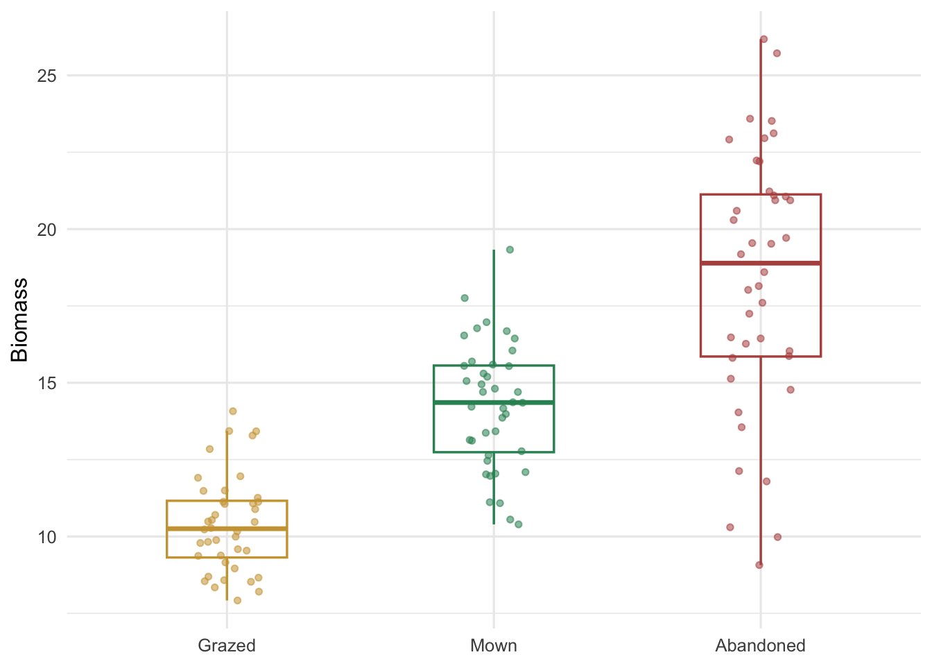
Three management types, forty plots each. The means differ, and so does the spread: grazed plots are tight, abandoned plots are roughly three times as variable.
```{r}
#| label: sim1
#| warning: false
#| message: false
library(nlme)

set.seed(7)
ng <- 40
mk <- function(level, mu, sdv) data.frame(mgmt = level, biomass = rnorm(ng, mu, sdv))
dat <- rbind(mk("Grazed", 10, 1.5), mk("Mown", 14, 2.2), mk("Abandoned", 18, 5.0))
dat$mgmt <- factor(dat$mgmt, levels = c("Grazed", "Mown", "Abandoned"))

round(tapply(dat$biomass, dat$mgmt, sd), 2)
bartlett.test(biomass ~ mgmt, data = dat)$p.value
```
The observed standard deviations are 1.57, 2.04 and 4.28, and Bartlett's test returns a p-value near 4e-10: the equal-variance hypothesis is firmly rejected. The picture is plainer than the test.
```{r}
#| label: fig-spread
#| fig-cap: "Biomass by management type. Spread grows from grazed to mown to abandoned, the unequal variance a single pooled estimate would paper over."
#| fig-alt: "Jittered points with boxplots for three management types; grazed is tightly clustered, mown wider, abandoned widest, with means also increasing."
#| warning: false
#| message: false
library(ggplot2)
mgmt_cols <- c(Grazed = "#cda23f", Mown = "#2f8f63", Abandoned = "#b5534e")

ggplot(dat, aes(mgmt, biomass, colour = mgmt)) +
  geom_jitter(width = 0.12, alpha = 0.55, size = 1.3) +
  geom_boxplot(fill = NA, outlier.shape = NA, width = 0.45, linewidth = 0.6) +
  scale_colour_manual(values = mgmt_cols, guide = "none") +
  labs(x = NULL, y = "Biomass") +
  theme_minimal(base_size = 12)
```
Fit two models with the same cell-means structure, differing only in the variance. The `varIdent(form = ~ 1 | mgmt)` weight gives each management type its own residual variance. Both are fitted with REML, so the AIC comparison is about the variance structure alone.
```{r}
#| label: fit1
#| warning: false
#| message: false
m0 <- gls(biomass ~ mgmt - 1, data = dat, method = "REML")
m1 <- gls(biomass ~ mgmt - 1, weights = varIdent(form = ~ 1 | mgmt),
          data = dat, method = "REML")

AIC(m0, m1)
anova(m0, m1)
```
Adding the per-group variance drops AIC from 598.9 to 559.3, about 40 units, and the likelihood-ratio test gives 43.6 on 2 degrees of freedom. The variance structure earns its two extra parameters several times over. Those parameters are interpretable: `varIdent` reports a multiplier per group, relative to the reference.
```{r}
#| label: varest
#| warning: false
#| message: false
m1$sigma # reference (Grazed) SD
coef(m1$modelStruct$varStruct, unconstrained = FALSE) # multipliers
```
The reference standard deviation is 1.57 (grazed), with multipliers of 1.30 for mown and 2.73 for abandoned, recovering group standard deviations of about 1.57, 2.04 and 4.28: the values the data showed. Now the part that matters for inference, the standard errors of the group means under each model.
```{r}
#| label: se1
#| warning: false
#| message: false
data.frame(mean        = coef(m1),
           SE_constant = sqrt(diag(vcov(m0))),
           SE_varIdent = sqrt(diag(vcov(m1))),
           row.names   = levels(dat$mgmt))
```
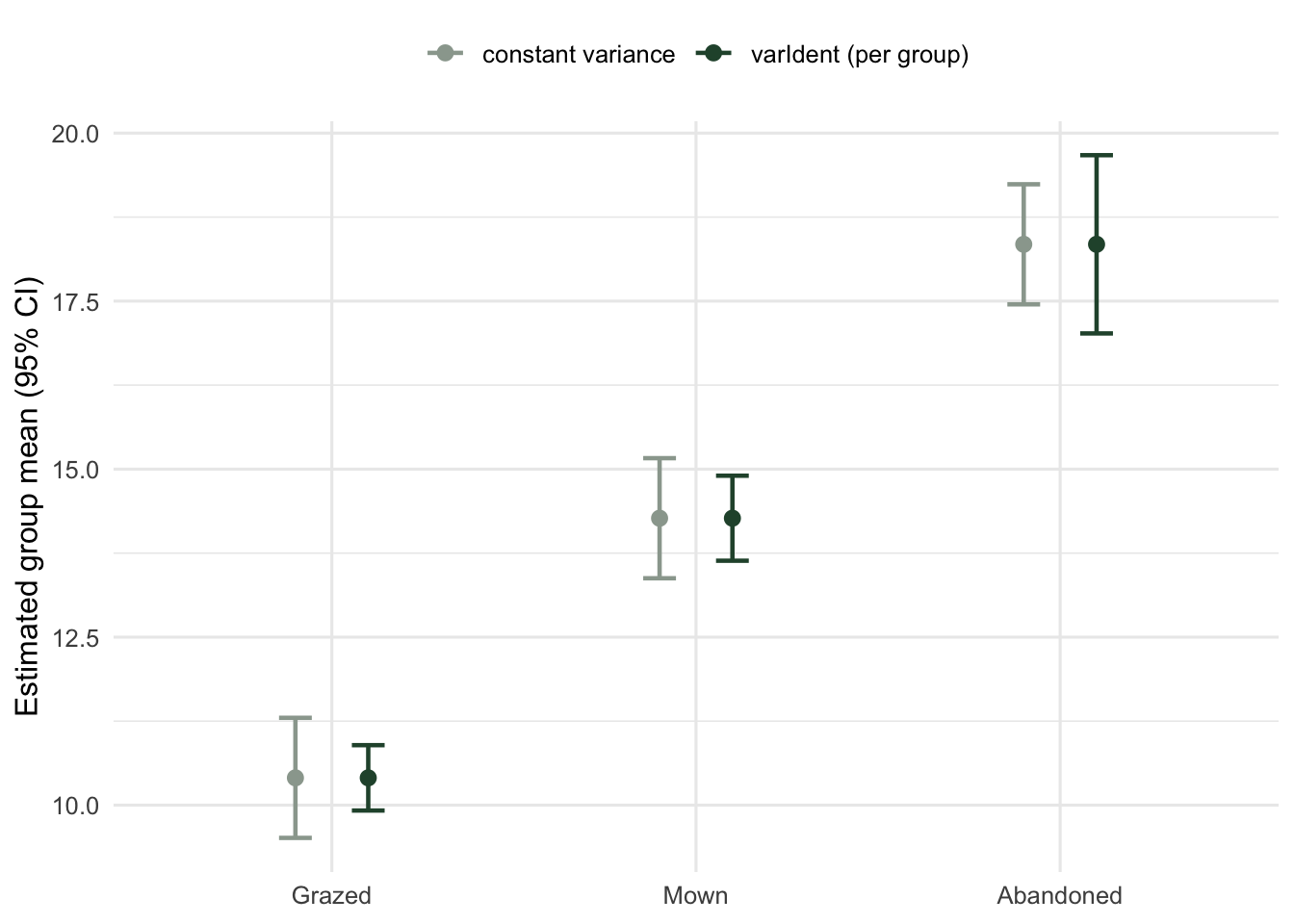
The constant-variance model assigns every group the same standard error, 0.46, because it has only one variance to share out and the groups are balanced. The `varIdent` model reports 0.25 for grazed, 0.32 for mown and 0.68 for abandoned. The means are essentially identical; the uncertainty is not. The pooled model understates the abandoned mean's error (0.46 against 0.68) and overstates the grazed mean's (0.46 against 0.25). The first is the dangerous direction: it claims more precision about the noisiest group than the data supports.
```{r}
#| label: fig-ci
#| fig-cap: "Group means with 95 percent intervals. Constant variance gives every group the same width; varIdent widens the noisy group and tightens the precise one, with the same point estimates."
#| fig-alt: "Estimated group means for three management types with 95 percent intervals under two models; constant-variance intervals are equal width, varIdent intervals are narrow for grazed and wide for abandoned."
#| warning: false
#| message: false
ci <- rbind(
  data.frame(mgmt = levels(dat$mgmt), model = "constant variance",
             mean = coef(m0), se = sqrt(diag(vcov(m0)))),
  data.frame(mgmt = levels(dat$mgmt), model = "varIdent (per group)",
             mean = coef(m1), se = sqrt(diag(vcov(m1)))))
ci$mgmt <- factor(ci$mgmt, levels = levels(dat$mgmt))
ci$lo <- ci$mean - 1.96 * ci$se
ci$hi <- ci$mean + 1.96 * ci$se

ggplot(ci, aes(mgmt, mean, colour = model)) +
  geom_point(position = position_dodge(0.4), size = 2.4) +
  geom_errorbar(aes(ymin = lo, ymax = hi), position = position_dodge(0.4),
                width = 0.18, linewidth = 0.8) +
  scale_colour_manual(values = c("constant variance" = "#9aa69d",
                                 "varIdent (per group)" = "#275139")) +
  labs(x = NULL, y = "Estimated group mean (95% CI)", colour = NULL) +
  theme_minimal(base_size = 12) +
  theme(legend.position = "top")
```
## Case two: variance grows with a predictor
The other common pattern is continuous: the scatter widens along a gradient. Here the residual standard deviation is proportional to a predictor `x`, so the variance grows with its square.
```{r}
#| label: sim2
#| warning: false
#| message: false
set.seed(31)
n <- 120
x <- runif(n, 1, 10)
y <- 2 + 1.2 * x + rnorm(n, 0, 0.35 * x)   # sd proportional to x
d2 <- data.frame(x = x, y = y)

m0 <- gls(y ~ x, data = d2, method = "REML")
m1 <- gls(y ~ x, weights = varPower(form = ~ x), data = d2, method = "REML")
AIC(m0, m1)
```
`varPower(form = ~ x)` models the variance as proportional to `|x|` raised to a power that the model estimates. AIC falls from 491.1 to 445.8. The estimated power and residual scale recover the truth.
```{r}
#| label: power-est
#| warning: false
#| message: false
coef(m1$modelStruct$varStruct, unconstrained = FALSE) # power
m1$sigma # scale
```
The estimated power is 0.98, against the true value of 1, and the scale is 0.33 against the 0.35 used to simulate. The variance function is right. This time the consequence runs the other way.
```{r}
#| label: slope2
#| warning: false
#| message: false
rbind(
  constant = summary(m0)$tTable["x", c("Value", "Std.Error")],
  varPower = summary(m1)$tTable["x", c("Value", "Std.Error")]
)
```
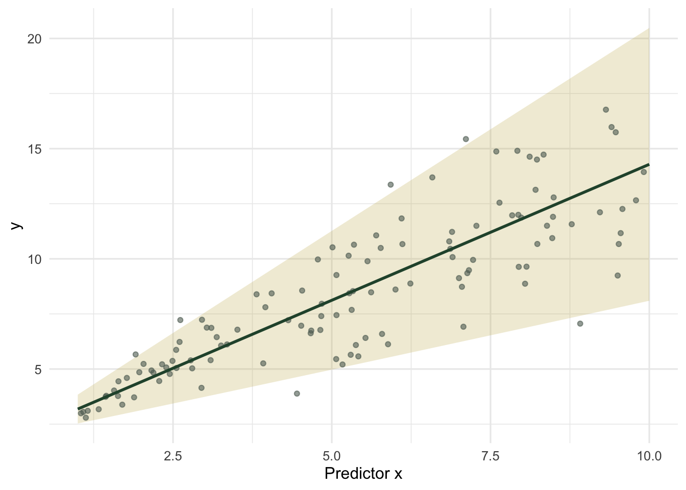
The constant-variance fit gives the slope a standard error of 0.065; the `varPower` fit gives 0.050. Modelling the variance made the slope *more* precise, not less. The reason is weighting: the high-`x` points are the noisy ones, and giving them equal weight wastes information. Downweighting them in proportion to their variance is the efficient thing to do, and it tightens the slope while nudging the estimate closer to the true 1.2. Case one widened a standard error and case two narrowed one. Both are the same act, replacing a wrong variance with the right one; the direction depends on where the noise sits.
```{r}
#| label: fig-funnel
#| fig-cap: "The varPower fit. The band is the mean plus or minus roughly two standard deviations from the estimated variance function, fanning out with x to match the data."
#| fig-alt: "Scatter of y against x with a green mean line and a gold band that widens as x increases, tracking the growing spread of the points."
#| warning: false
#| message: false
delta <- coef(m1$modelStruct$varStruct, unconstrained = FALSE)
gx <- seq(1, 10, length = 100)
band <- data.frame(x = gx, fit = coef(m1)[1] + coef(m1)[2] * gx,
                   sd = m1$sigma * gx^delta)

ggplot(d2, aes(x, y)) +
  geom_ribbon(data = band, aes(x = x, ymin = fit - 1.96 * sd, ymax = fit + 1.96 * sd),
              inherit.aes = FALSE, fill = "#c9b458", alpha = 0.25) +
  geom_point(colour = "#5d6b61", alpha = 0.6, size = 1.4) +
  geom_line(data = band, aes(x, fit), inherit.aes = FALSE,
            colour = "#275139", linewidth = 1) +
  labs(x = "Predictor x", y = "y") +
  theme_minimal(base_size = 12)
```
## Choosing and checking a structure
Match the function to the pattern. `varIdent` is for categorical strata with different spreads: sites, treatments, sexes, years. `varPower` and `varExp` are for variance that changes smoothly with a covariate or with the fitted values themselves (`form = ~ fitted(.)`), the power form for variance that scales with a quantity and the exponential form when the variance keeps climbing where a power law would flatten. `varConstPower` adds a floor for data that has a baseline variance plus a growing part.
The diagnostic that flags the problem also checks the cure: plot the standardised residuals against fitted values and against any candidate grouping or covariate. A fan or a block of unequal spread signals trouble before fitting, and after fitting a good variance structure the standardised residuals should sit in an even band. The same `weights` argument works inside `lme`, so everything here carries straight into the mixed models from the [random slopes post](../random-slopes-mixed-models/), and it composes with the correlation structures from the [spatial GLS post](../gls-spatial-correlation/): a model can carry a variance function and a correlation structure at once.
## References
Pinheiro JC, Bates DM 2000. Mixed-Effects Models in S and S-PLUS. Springer (ISBN 978-0-387-98957-0)
Zuur AF, Ieno EN, Walker NJ, Saveliev AA, Smith GM 2009. Mixed Effects Models and Extensions in Ecology with R. Springer (ISBN 978-0-387-87457-9)
## Related tutorials
- [Repeated measures and temporal correlation](../repeated-measures-temporal-correlation/)
- [Marginal vs conditional R-squared](../marginal-vs-conditional-r2/)
- [Random slopes in mixed models](../random-slopes-mixed-models/)
- [GLS for spatial correlation](../gls-spatial-correlation/)