---
title: "Marginal and conditional R-squared for mixed models"
description: "A mixed model has two R-squared values: marginal for the fixed effects, conditional for fixed plus random. Compute both by hand in R from an nlme model."
date: "2026-06-30 21:00"
categories: [mixed models, R, nlme, model evaluation, ecology tutorial]
image: thumbnail.png
image-alt: "A single horizontal bar splitting total variance into fixed, random and residual parts, with markers for marginal and conditional R-squared."
---
A linear model has one R-squared: the share of variance the predictors account for. A mixed model has two answers to that question, because it explains variance in two different ways. The fixed effects explain some of it directly. The grouping structure, the random effects, explains more by letting each site or individual sit at its own level. Quote a single R-squared and you have hidden which kind you mean.
Nakagawa and Schielzeth (2013) gave the two numbers names. Marginal R-squared is the variance explained by the fixed effects alone. Conditional R-squared is the variance explained by the fixed and random effects together. Both are worth reporting, they answer different questions, and neither needs a package: each is built from three variances the fitted model already contains.
## The three variances
Take the random-intercept model from the [random slopes post](../random-slopes-mixed-models/) family: a response driven by a predictor, with a site-level intercept. Three quantities describe where its variance lives. The fixed-effects variance is the spread of the predictions made from the fixed part alone, the variation the predictors generate across the data. The random-effects variance is the spread of the site intercepts. The residual variance is what is left within sites. Marginal R-squared puts the fixed-effects variance over the total of all three; conditional R-squared puts the fixed plus random over the same total.
Simulate a clean case: twenty sites, ten observations each, one predictor, a site intercept, Gaussian noise.
```{r}
#| label: sim
#| warning: false
#| message: false
library(nlme)

set.seed(44)
nsite <- 20; nrep <- 10
site <- factor(rep(sprintf("S%02d", 1:nsite), each = nrep))
a <- rnorm(nsite, 0, 2)                  # site intercepts
x <- rnorm(nsite * nrep, 0, 1)
y <- 5 + 1.5 * x + a[as.integer(site)] + rnorm(nsite * nrep, 0, 1.5)
dat <- data.frame(site = site, x = x, y = y)

m <- lme(y ~ x, random = ~ 1 | site, data = dat, method = "REML")
summary(m)$tTable
```
The slope is estimated at 1.52 with a t-value above 14: as significant as effects come. Hold that in mind, because significance and variance explained are about to part ways.
## Pulling out the components
Each variance is one line. The fixed-effects variance is the variance of the marginal predictions, those made at `level = 0`, which use only the fixed effects. The random-intercept variance comes straight from `VarCorr`. The residual is `sigma(m)` squared.
```{r}
#| label: components
#| warning: false
#| message: false
var_f <- var(as.vector(predict(m, level = 0)))          # fixed effects
var_a <- as.numeric(VarCorr(m)["(Intercept)", "Variance"])  # random intercept
var_e <- sigma(m)^2                                     # residual

c(fixed = var_f, random = var_a, residual = var_e)
```
The fixed effects carry a variance of 2.48, the site intercepts 6.09, the residual 2.27. The grouping is the largest single source here, which already hints at the answer.
```{r}
#| label: r2
#| warning: false
#| message: false
total <- var_f + var_a + var_e
R2_marginal    <- var_f / total
R2_conditional <- (var_f + var_a) / total

c(marginal = R2_marginal, conditional = R2_conditional)
```
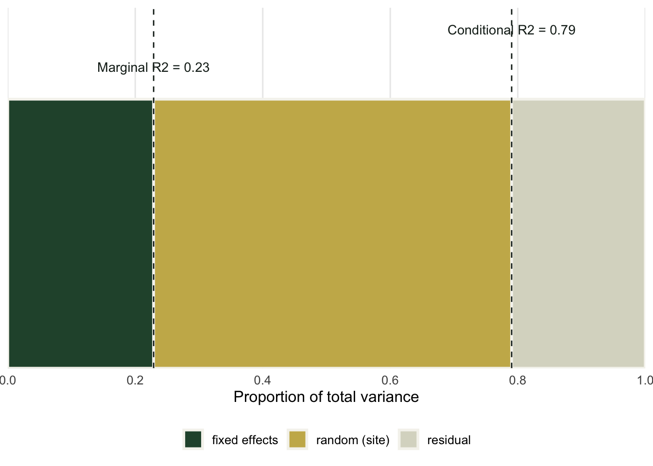
Marginal R-squared is 0.23; conditional R-squared is 0.79. The picture is the whole story: the bar is total variance, split into the three parts, with the two R-squared values reading off as cumulative shares from the left.
```{r}
#| label: fig-decomp
#| fig-cap: "Total variance split into fixed, random and residual. Marginal R-squared is the fixed share; conditional R-squared adds the random share. The residual is the part neither explains."
#| fig-alt: "A horizontal bar from zero to one split into a green fixed segment to 0.23, a gold random segment to 0.79, and a pale residual segment to one, with dashed markers at the two R-squared values."
#| warning: false
#| message: false
library(ggplot2)

ord <- data.frame(part = c("fixed effects", "random (site)", "residual"),
                   frac = c(var_f, var_a, var_e) / total)
ord$xmin <- c(0, cumsum(ord$frac)[-3])
ord$xmax <- cumsum(ord$frac)
ord$part <- factor(ord$part, levels = ord$part)
cols <- c("fixed effects" = "#275139", "random (site)" = "#c9b458",
          "residual" = "#dad9ca")

ggplot(ord) +
  geom_rect(aes(xmin = xmin, xmax = xmax, ymin = 0, ymax = 1, fill = part),
            colour = "#f5f4ee", linewidth = 1) +
  scale_fill_manual(values = cols, name = NULL) +
  geom_vline(xintercept = R2_marginal,    colour = "#16241d",
             linewidth = 0.5, linetype = "dashed") +
  geom_vline(xintercept = R2_conditional, colour = "#16241d",
             linewidth = 0.5, linetype = "dashed") +
  annotate("text", x = R2_marginal, y = 1.12,
           label = sprintf("Marginal R2 = %.2f", R2_marginal),
           hjust = 0.5, size = 3.6, colour = "#16241d") +
  annotate("text", x = R2_conditional, y = 1.26,
           label = sprintf("Conditional R2 = %.2f", R2_conditional),
           hjust = 0.5, size = 3.6, colour = "#16241d") +
  scale_x_continuous(limits = c(0, 1), breaks = seq(0, 1, 0.2), expand = c(0, 0)) +
  scale_y_continuous(limits = c(0, 1.34), expand = c(0, 0)) +
  labs(x = "Proportion of total variance", y = NULL) +
  theme_minimal(base_size = 12) +
  theme(axis.text.y = element_blank(), panel.grid.major.y = element_blank(),
        panel.grid.minor = element_blank(), legend.position = "bottom")
```
## What the two numbers say
The predictor has a slope that is overwhelmingly significant, yet it accounts for only 23 percent of the total variance. That is not a contradiction. Significance is about whether the slope is distinguishable from zero; marginal R-squared is about how much of the spread in the data that slope explains. A small but precisely estimated effect can be both real and minor, and reporting only the p-value hides the second half.
The jump from 0.23 to 0.79 is the site structure. Most of the explainable variation here is not the predictor at all; it is that sites differ from one another, captured by the random intercept. The gap between the two R-squared values is itself informative: a wide gap means the grouping carries most of the signal, a narrow one means the fixed effects do. Reporting both keeps that honest. A model can look weak by marginal R-squared and strong by conditional, and a reader deserves to see which.
## Scope and extensions
This three-variance recipe is exact for a Gaussian random-intercept model. Two cases need more care. With random slopes the random-effects variance is no longer a single intercept variance; it depends on the values of the predictor, and Johnson (2014) gives the extension that handles it. For non-Gaussian responses (a Poisson or binomial GLMM) the residual variance is not directly available and a distribution-specific term enters on the link scale, worked out in the 2017 follow-up by the same authors.
Packages compute these for you: `performance::r2_nakagawa` and `MuMIn::r.squaredGLMM` both return the pair. The point of doing it by hand once is to know what they return. A marginal and a conditional R-squared are not a fixed property of the data; they are a statement about how variance is split between what you measured and the structure you grouped by, and seeing the three pieces add up makes that split concrete.
## References
Nakagawa S, Schielzeth H 2013. Methods in Ecology and Evolution 4(2):133-142 (10.1111/j.2041-210x.2012.00261.x)
Johnson PCD 2014. Methods in Ecology and Evolution 5(9):944-946 (10.1111/2041-210X.12225)
## Related tutorials
- [Model selection and AIC](../model-selection-aic/)
- [Variance structure and heteroscedasticity](../variance-structure-heteroscedasticity/)
- [Repeated measures and temporal correlation](../repeated-measures-temporal-correlation/)
- [Random slopes in mixed models](../random-slopes-mixed-models/)