---
title: "Random slopes in mixed models with nlme"
description: "When the effect of a predictor varies between sites, random intercepts are not enough. Fit and interpret random slopes in R with nlme, including shrinkage."
date: "2026-06-30 18:00"
categories: [mixed models, R, nlme, regression, ecology tutorial]
image: thumbnail.png
image-alt: "Site-specific regression lines fanning out around a population slope, with a shrinkage plot showing per-site slopes pulled toward the mean."
---
A random intercept lets every group sit at its own height. The slope, the rate at which the response changes with a predictor, is held common across all groups: parallel lines at different elevations. That is often the right starting point, and the [pseudoreplication post](../pseudoreplication-in-ecology/) used exactly this structure to recover the correct uncertainty for a between-group treatment.
The assumption breaks when groups respond *differently* to the predictor. If nutrient addition boosts growth steeply at some sites and barely at others, a single fixed slope is the wrong summary, and forcing one has a specific cost: the standard error of that average slope comes out too small. Schielzeth and Forstmeier (2009) showed this leads to overconfident conclusions across a swathe of the behavioural ecology literature. A random slope is the fix. This post builds the case on data where the truth is known.
## A gradient measured across sites
Twelve sites, eight plots each, growth measured against a centred nutrient gradient. The site intercepts and site slopes are drawn together from a bivariate normal, so a site that starts high tends to respond more gently (a negative intercept-slope correlation built into the truth).
```{r}
#| label: simulate
#| warning: false
#| message: false
library(nlme)

set.seed(20)
nsite <- 12
nrep  <- 8
sites <- factor(sprintf("S%02d", 1:nsite))

sd_int <- 3.0; sd_slope <- 1.3; rho <- -0.45; sd_resid <- 1.6
Sigma <- matrix(c(sd_int^2,            rho*sd_int*sd_slope,
                  rho*sd_int*sd_slope, sd_slope^2), 2, 2)
z   <- matrix(rnorm(nsite * 2), nsite, 2) %*% chol(Sigma)
b0i <- 10 + z[, 1]   # site intercepts
b1i <- 2  + z[, 2]   # site slopes (population slope = 2)

dat <- do.call(rbind, lapply(1:nsite, function(i) {
  x <- round(runif(nrep, -2, 2), 2)
  y <- b0i[i] + b1i[i] * x + rnorm(nrep, 0, sd_resid)
  data.frame(site = sites[i], nutrient = x, growth = y)
}))

c(rows = nrow(dat), sites = nlevels(dat$site))
```
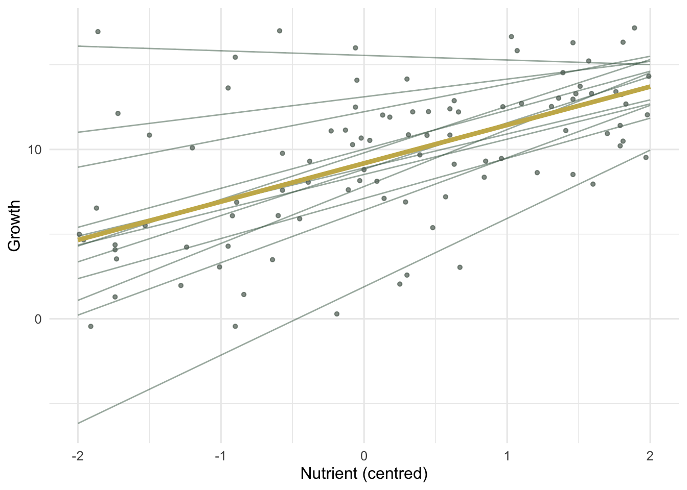
The fanning is visible before any model is fitted: per-site regression lines differ in slope, not just height, and the steeper-starting sites tend to flatten out.
```{r}
#| label: fig-spaghetti
#| fig-cap: "Per-site fitted lines from the random-slopes model (thin) around the population line (thick gold). Slopes differ in steepness, and high-intercept sites tend to be shallower."
#| fig-alt: "Scatter of growth against centred nutrient with twelve thin site lines of differing slope and a thick gold population line through the middle; one site line has a negative slope."
#| warning: false
#| message: false
library(ggplot2)

m_slope <- lme(growth ~ nutrient, random = ~ nutrient | site,
               data = dat, method = "REML")

grid <- expand.grid(nutrient = c(-2, 2), site = levels(dat$site))
grid$fit <- predict(m_slope, newdata = grid)
pop <- data.frame(nutrient = c(-2, 2))
pop$fit <- fixef(m_slope)[1] + fixef(m_slope)[2] * pop$nutrient

ggplot(dat, aes(nutrient, growth)) +
  geom_line(data = grid, aes(y = fit, group = site),
            colour = "#275139", alpha = 0.45, linewidth = 0.5) +
  geom_point(colour = "#5d6b61", size = 1.1, alpha = 0.7) +
  geom_line(data = pop, aes(y = fit), colour = "#c9b458", linewidth = 1.6) +
  labs(x = "Nutrient (centred)", y = "Growth") +
  theme_minimal(base_size = 12)
```
## Intercept only versus intercept and slope
Two models, identical fixed part, differing only in what the site is allowed to vary. Both are fitted with REML, which keeps the variance-component estimates comparable because the fixed-effects structure is the same.
```{r}
#| label: fit-compare
#| warning: false
#| message: false
m_int   <- lme(growth ~ nutrient, random = ~ 1        | site,
               data = dat, method = "REML")
m_slope <- lme(growth ~ nutrient, random = ~ nutrient | site,
               data = dat, method = "REML")

AIC(m_int, m_slope)
anova(m_int, m_slope)
```
The random-slopes model has an AIC of 435.8 against 461.6 for the intercept-only model, an improvement of about 26 units. The likelihood-ratio test gives a statistic of 29.9 on 2 degrees of freedom. One caution on that test: a variance of zero sits on the boundary of the parameter space, so the usual chi-squared reference distribution is conservative here, and the true p-value is even smaller than reported. With a gap this size the conclusion is not in doubt, but for borderline cases the AIC comparison is the safer guide.
## Reading the variance components
`VarCorr` reports the spread of the random effects on the standard-deviation scale, which is the scale to interpret.
```{r}
#| label: varcorr
#| warning: false
#| message: false
VarCorr(m_slope)
```
Site intercepts have a standard deviation of 3.55 and site slopes 1.22, against a population slope of about 2.26. A slope spread of 1.22 around a mean of 2.26 is large: it says the nutrient effect is genuinely heterogeneous, not a fixed quantity blurred by noise. The estimated intercept-slope correlation is -0.85, the negative relationship that was built into the data, though correlations of random effects are poorly pinned down with only twelve groups and this estimate should be read as approximate. The residual standard deviation is 1.71.
## The cost of forcing a common slope
The headline consequence is the standard error of the fixed slope. Pull it from both models.
```{r}
#| label: se-cost
#| warning: false
#| message: false
rbind(
  intercept_only = summary(m_int)$tTable["nutrient",   c("Value", "Std.Error")],
  random_slopes  = summary(m_slope)$tTable["nutrient", c("Value", "Std.Error")]
)
```
The intercept-only model reports the average slope with a standard error of 0.21. The random-slopes model reports a standard error of 0.40 for essentially the same estimate. The error nearly doubles. This is the Schielzeth and Forstmeier point made concrete: the parallel-lines model treats all 96 plots as independent evidence about one slope, when the real replication is twelve sites with their own slopes. Ignore the slope variation and the precision is overstated, which is exactly how a true effect gets reported as more certain than the data can support.
## Shrinkage: partial pooling toward the mean
A random-slopes model does not return the twelve separate within-site regressions. It returns slopes pulled toward the population value, with the pull stronger for sites whose own estimate is extreme or poorly supported. Compare the per-site OLS slopes with the model's per-site slopes.
```{r}
#| label: fig-shrinkage
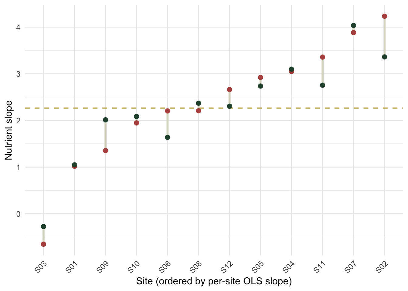
#| fig-cap: "Per-site slopes: independent OLS estimates (rust) and the model's partially pooled estimates (green), connected. The dashed gold line is the population slope. Extreme OLS slopes are pulled inward."
#| fig-alt: "Twelve sites ordered by OLS slope; rust points show OLS slopes, green points the pooled estimates, joined by grey segments; both extremes move toward a dashed gold horizontal line at the population slope."
#| warning: false
#| message: false
ols  <- sapply(levels(dat$site),
               function(s) coef(lm(growth ~ nutrient, dat[dat$site == s, ]))["nutrient"])
blup <- coef(m_slope)[, "nutrient"]
pop_slope <- fixef(m_slope)["nutrient"]

sh <- data.frame(site = levels(dat$site),
                 ols = as.numeric(ols), blup = as.numeric(blup))
sh <- sh[order(sh$ols), ]
sh$site <- factor(sh$site, levels = sh$site)

c(pop_slope = round(pop_slope, 3),
  sd_ols = round(sd(sh$ols), 3), sd_blup = round(sd(sh$blup), 3))
ggplot(sh) +
  geom_hline(yintercept = pop_slope, colour = "#c9b458",
             linetype = "dashed", linewidth = 0.7) +
  geom_segment(aes(x = site, xend = site, y = ols, yend = blup),
               colour = "#dad9ca", linewidth = 1.2) +
  geom_point(aes(site, ols),  colour = "#b5534e", size = 2.3) +
  geom_point(aes(site, blup), colour = "#275139", size = 2.3) +
  labs(x = "Site (ordered by per-site OLS slope)", y = "Nutrient slope") +
  theme_minimal(base_size = 12) +
  theme(axis.text.x = element_text(angle = 45, hjust = 1))
```
The spread of slopes drops from 1.34 across the independent OLS fits to 1.13 across the pooled estimates. The sites near the population value barely move; the two extremes, one near 4.2 and one slightly negative, are pulled noticeably toward the centre. This is partial pooling: each site borrows strength from the others, so a single odd site does not get to claim an extreme slope on thin evidence. It is the same mechanism that makes mixed-model predictions more stable than twelve separate regressions.
## Practical notes
Centre the predictor before fitting. With `nutrient` centred, the intercept variance is the spread of sites at the gradient mean and the intercept-slope correlation is interpretable; on a raw scale both shift with the arbitrary zero.
Random slopes ask a lot of the data. The between-group variance components, and the intercept-slope correlation in particular, need a reasonable number of groups to estimate; with very few sites the slope variance tends to be underestimated and the model can fail to converge. If `lme` does not converge, fitting the intercept and slope variances without their correlation (a diagonal random-effects structure) is the usual first simplification.
Include a random slope for a predictor whenever its effect could plausibly vary across the grouping unit and that variation is part of the question. The test is design and biology, not the p-value: if sites, individuals, or plots might respond at different rates, the average-rate standard error from an intercept-only model is the one to distrust.
## References
Schielzeth H, Forstmeier W 2009. Behavioral Ecology 20(2):416-420 (10.1093/beheco/arn145)
Pinheiro JC, Bates DM 2000. Mixed-Effects Models in S and S-PLUS. Springer (ISBN 978-0-387-98957-0)
## Related tutorials
- [GLS for spatial correlation](../gls-spatial-correlation/)
- [Repeated measures and temporal correlation](../repeated-measures-temporal-correlation/)
- [GLMMs for nested counts](../glmm-nested-counts-pseudoreplication/)
- [Variance structure and heteroscedasticity](../variance-structure-heteroscedasticity/)