library(ggplot2)

te_pal <- list(forest = "#275139", green = "#2f8f63", sage = "#93a87f",
               clay = "#b5534e", gold = "#cda23f", line = "#dad9ca",
               ink = "#16241d", paper = "#f5f4ee")

fmt <- function(x, digits = 4) formatC(x, format = "f", digits = digits)

theme_te <- function() {
  theme_minimal(base_size = 12) +
    theme(panel.grid.minor = element_blank(),
          panel.grid.major = element_line(colour = "#e7e6dc"),
          plot.background = element_rect(fill = "#f5f4ee", colour = NA),
          panel.background = element_rect(fill = "#f5f4ee", colour = NA),
          plot.title = element_text(face = "bold", colour = te_pal$ink),
          axis.title = element_text(colour = "#2c3a31"),
          legend.position = "bottom")
}Checking a mixture model
R
mixture models
model checking
ecology tutorial
Four measured checks on a fitted finite mixture in R: multiple optima, classification versus parameter uncertainty, the unbounded likelihood and predictive fit.
The gill nets came out of the lake at seven in the morning and the whole catch went onto a measuring board before the ice in the bins gave up. By ten there were two hundred fork lengths in a notebook, and by the afternoon a histogram on a laptop in the hut: a tall clump near ten and a half centimetres, a shoulder just above it that might or might not be a second clump, a clear trough, and a broad hump near sixteen.
The point was to age the catch without reading a single otolith. Fish that hatched in the same summer grow together, so a length frequency from one survey is a sum of cohort-specific distributions, and pulling the sum apart gives the cohort sizes for free. That is a finite mixture, and fitting one is a short loop in base R. The fitting is not the hard part.
The hard part is that the fitted object hands back numbers with no warning label on any of them. It reports three component means to four decimal places whether or not there are three cohorts in the lake. It reports a posterior probability that a fish belongs to the middle cohort even when that probability is a coin toss. It reports the same log-likelihood from a run that found the best solution and from a run that found a different one with the labels shuffled.
This post runs four checks on a fitted mixture, each a measurement against a truth that is known because the data were simulated, and each able to change what you would report from a real survey. Three of the four came back against the expectation they were written from, and in every case the measurement was kept and the section rebuilt around it: the most popular solution across random starts is not the best one, the posterior membership weights everybody recommends are more biased than the hard assignment they replace, and the equal-variance constraint that is the standard cure for a degenerate fit buys nothing over doing nothing at all.
If the machinery is new, fitting a mixture of normals in R builds the same EM fitter from scratch, how many components in a mixture? is about choosing the number of components rather than checking a chosen one, and when a mixture is really skewness asks whether a mixture is the right shape at all. Everything below is base R plus ggplot2, a few hundred replicates per measurement, and under a minute of knitting.
The fitter, written out once
All four checks use the same expectation maximisation loop, so it belongs on the page rather than behind a package call. The E step turns the current parameters into a matrix of membership weights, one row per fish and one column per component; the M step treats those weights as counts and does weighted means and weighted variances. The log-likelihood is computed inside the E step, before the parameters move, so the value returned belongs to the parameters current at the last iteration.
em_mix <- function(x, K, mu, sdev, prop, maxit = 800, tol = 1e-9,
                   sd_floor = 0, equal_var = FALSE, pen_a = 0) {
  n <- length(x)
  sx2 <- sum((x - mean(x))^2) / n
  ll_old <- -Inf; ll <- -Inf; it <- 0L
  logd <- matrix(0, n, K); z <- matrix(0, n, K)
  for (it in seq_len(maxit)) {
    for (k in seq_len(K)) logd[, k] <- log(prop[k]) + dnorm(x, mu[k], sdev[k], log = TRUE)
    mx <- logd[, 1]
    if (K > 1) for (k in 2:K) mx <- pmax(mx, logd[, k])
    w <- exp(logd - mx)
    rs <- rowSums(w)
    ll <- sum(log(rs)) + sum(mx)
    if (pen_a > 0) ll <- ll - pen_a * sum(sx2 / sdev^2 + log(sdev^2))
    z <- w / rs
    if (is.finite(ll) && abs(ll - ll_old) < tol) break
    ll_old <- ll
    nk <- colSums(z); prop <- nk / n
    mu <- as.numeric(crossprod(z, x)) / nk
    ss <- numeric(K)
    for (k in seq_len(K)) ss[k] <- sum(z[, k] * (x - mu[k])^2)
    sdev <- if (equal_var) rep(sqrt(sum(ss) / n), K) else
      sqrt((ss + 2 * pen_a * sx2) / (nk + 2 * pen_a))
    if (sd_floor > 0) sdev <- pmax(sdev, sd_floor)
  }
  list(mu = mu, sd = sdev, prop = prop, loglik = ll, iter = it, z = z)
}

rmix <- function(n, mu, sdev, prop) {
  k <- sample(seq_along(mu), n, TRUE, prop)
  rnorm(n, mu[k], sdev[k])
}
rand_start <- function(x, K, lo = 0.4, hi = 1.4) {
  list(mu = sample(x, K), sdev = sd(x) * runif(K, lo, hi), prop = rep(1 / K, K))
}
Three arguments in the signature do nothing yet and exist for the third check. sd_floor refuses to let any component standard deviation fall below a stated value. equal_var pools the weighted sums of squares so every component shares one standard deviation. pen_a adds a penalty to the log-likelihood that punishes small variances, and it changes the M step too, because the penalised update adds pseudo-observations of the overall spread to every component. The first two constrain the parameter space; the third changes the objective.
rand_start is the crude but honest way to start a mixture fit: pick K observed values as the initial means, give every component a random multiple of the overall spread, split the weight evenly. Starting from a k-means partition or from quantiles hides the behaviour the first check is about, because a clever start lands in the same place every time.
The convergence rule stops when the increase in the log-likelihood falls below tol. EM on an overlapping mixture converges linearly and slowly, so a loose tolerance stops runs while the parameters are still moving, which then looks like a forest of distinct solutions that are really one solution seen at different stages. Every count of optima below uses a very tight tolerance and an iteration cap no run reaches.
Check one: which optimum did the run find
The mixture likelihood is symmetric in the components. Relabel component one as component three and the density is unchanged, so with three components there are six parameter vectors that give exactly the same fit and exactly the same log-likelihood. Averaging over runs, or over MCMC draws, without doing something about that symmetry produces an average of six different things.
That is the easy half. The hard half is that a run ending somewhere else entirely also returns a log-likelihood, and from the parameters alone it can be hard to tell a relabelled copy of the best solution from a genuinely worse one that looks similar. The measurement below separates them: relabel by sorting on the component mean, group what is left by log-likelihood, then check whether the relabelled parameters inside a group agree.
set.seed(20260729)
mu_a <- c(10.5, 12.0, 16.0); sd_a <- c(0.6, 0.6, 1.0); p_a <- c(0.25, 0.25, 0.50)
n_a <- 200; K_a <- 3; starts_a <- 120
x_a <- rmix(n_a, mu_a, sd_a, p_a)
floor_a <- 0.1 * sd(x_a)

print(round(c(n = n_a, components = K_a, starts = starts_a, sd_floor = floor_a), 4))
n components starts sd_floor
200.0000 3.0000 120.0000 0.2569 print(round(c(mu_1 = mu_a[1], mu_2 = mu_a[2], mu_3 = mu_a[3],
sd_1 = sd_a[1], sd_2 = sd_a[2], sd_3 = sd_a[3],
w_1 = p_a[1], w_2 = p_a[2], w_3 = p_a[3],
young_separation_sd = (mu_a[2] - mu_a[1]) / sd_a[1]), 4)) mu_1 mu_2 mu_3 sd_1
10.50 12.00 16.00 0.60
sd_2 sd_3 w_1 w_2
0.60 1.00 0.25 0.25
w_3 young_separation_sd
0.50 2.50 The simulated survey is 200 fish from three cohorts. Two are young and tightly graded, at 10.5 and 12.0 centimetres with a standard deviation of 0.6, holding a quarter of the catch each. The third is everything older, centred at 16.0 centimetres with a standard deviation of 1.0 and half the weight. The young pair sit 2.5000 standard deviations apart, close enough that a histogram shows a shoulder rather than two peaks. A floor on the component standard deviations of 0.2569 centimetres is in force, for reasons the third check makes clear.
raw_a <- matrix(NA_real_, starts_a, K_a)
ord_a <- matrix(NA_real_, starts_a, 3 * K_a)
ll_a <- numeric(starts_a); it_a <- numeric(starts_a)

for (r in seq_len(starts_a)) {
  st <- rand_start(x_a, K_a)
  f <- em_mix(x_a, K_a, st$mu, st$sdev, st$prop, maxit = 1500, tol = 1e-10,
              sd_floor = floor_a)
  raw_a[r, ] <- f$mu
  o <- order(f$mu)
  ord_a[r, ] <- c(f$mu[o], f$sd[o], f$prop[o])
  ll_a[r] <- f$loglik; it_a[r] <- f$iter
}
print(round(c(mean_iterations = mean(it_a), max_iterations = max(it_a),
              total_iterations = sum(it_a)), 1))
mean_iterations max_iterations total_iterations
340.9 622.0 40905.0 raw_a keeps the component means in whatever order the fitter left them and ord_a keeps the same solution sorted by mean, the standard ordering constraint. Storing both is the whole trick: what differs between them is label switching, what survives the sorting is not.
The 120 runs took 40905 EM iterations between them, an average of 340.9 per run, the slowest needing 622. EM is often described as fast, and on well separated components it is, but these two young cohorts overlap enough that the membership weights barely move from one iteration to the next. A run stopped after fifty iterations would look converged and would not be.
ll_tol <- 0.05
grp_a <- integer(starts_a); n_opt <- 0L; last <- Inf
ranked <- order(ll_a, decreasing = TRUE)
for (i in ranked) {
  if (last - ll_a[i] > ll_tol) { n_opt <- n_opt + 1L; last <- ll_a[i] }
  grp_a[i] <- n_opt
}
first_of <- vapply(seq_len(n_opt), function(j) which(grp_a == j)[1], 1L)
opt_tab <- data.frame(optimum = seq_len(n_opt),
  logLik = round(vapply(seq_len(n_opt), function(j) max(ll_a[grp_a == j]), 0), 4),
  share_of_starts = round(as.numeric(table(grp_a)) / starts_a, 4),
  round(ord_a[first_of, , drop = FALSE], 3))
names(opt_tab)[4:12] <- c("mu_1", "mu_2", "mu_3", "sd_1", "sd_2", "sd_3",
                          "w_1", "w_2", "w_3")
print(opt_tab)
optimum logLik share_of_starts mu_1 mu_2 mu_3 sd_1 sd_2 sd_3
1 1 -405.7513 0.3417 10.571 12.165 15.841 0.615 0.519 0.955
2 2 -407.9671 0.4917 11.102 15.701 17.635 0.974 0.787 0.411
3 3 -408.4279 0.1667 11.086 15.596 15.929 0.959 0.457 1.066
w_1 w_2 w_3
1 0.328 0.153 0.519
2 0.485 0.472 0.043
3 0.482 0.135 0.384gap_a <- opt_tab$logLik[1] - opt_tab$logLik[2]
print(round(c(grouping_tolerance = ll_tol, n_optima = n_opt, logLik_gap = gap_a,
percent_best = 100 * opt_tab$share_of_starts[1],
percent_runner_up = 100 * opt_tab$share_of_starts[2]), 4))grouping_tolerance n_optima logLik_gap percent_best
0.0500 3.0000 2.2158 34.1700
percent_runner_up
49.1700 The grouping rule is deliberately crude: sort the runs by log-likelihood and start a new group whenever the drop from the previous run exceeds 0.05. Solutions closer than that are not practically distinguishable, and grouping them avoids counting numerical dust as structure.
3 groups came out of 120 runs. The best has a log-likelihood of -405.7513 and component means of 10.571, 12.165 and 15.841 centimetres against a truth of 10.5, 12.0 and 16.0. It is the only solution that splits the young clump into two cohorts, and it splits it unevenly: the weights come back as 0.328 and 0.153 when both are truly 0.25, which is what two hundred fish buy on a pair of components this close together.
Now the part that was not in the plan. The best solution was reached by 34.17 per cent of the starts; the second, worse by 2.2158 in log-likelihood, by 49.17 per cent. The plurality answer is not the maximum likelihood answer. Taking the solution that comes up most often, on the reasonable-sounding grounds that a repeatable answer is a stable one, would have given means of 11.102, 15.701 and 17.635 centimetres, the two young cohorts merged into one broad component and a spare narrow component parked at the top holding a weight of 0.043.
The size of a basin has nothing to do with the height of its peak. Random starts sample basins, not peaks, and a wide shallow basin catches more of them than a narrow tall one. Keep the best run rather than the commonest, and do enough runs that the best value stops improving.
best_a <- which(grp_a == 1)
perm_a <- apply(raw_a[best_a, ], 1, function(v) paste(order(v), collapse = ""))
spread_a <- max(apply(ord_a[best_a, ], 2, function(v) diff(range(v))))

print(round(c(runs_at_best = length(best_a),
              label_orders_seen = length(unique(perm_a))), 4))
runs_at_best label_orders_seen
41 6 print(signif(c(largest_parameter_range = spread_a), 2))largest_parameter_range
2.6e-05 print(round(c(raw_mean_1 = mean(raw_a[best_a, 1]), raw_mean_2 = mean(raw_a[best_a, 2]),
raw_mean_3 = mean(raw_a[best_a, 3]),
ordered_mean_1 = mean(ord_a[best_a, 1]),
ordered_mean_2 = mean(ord_a[best_a, 2]),
ordered_mean_3 = mean(ord_a[best_a, 3])), 4)) raw_mean_1 raw_mean_2 raw_mean_3 ordered_mean_1 ordered_mean_2
12.7744 12.9267 12.8759 10.5712 12.1652
ordered_mean_3
15.8406 The diagnosis is short. 41 runs reached the best optimum, and all 6 possible orderings of three components appeared among them. After sorting by the component mean, the largest range over any of the nine parameters is 2.6e-05. These are not similar solutions; they are one solution written down six ways.
The consequence is in the last block. Averaging the first stored component mean over those runs gives 12.7744 centimetres, the second 12.9267, the third 12.8759. All three are close to each other and none is a cohort: each slot receives each of the three components about equally often, so each average estimates the unweighted mean of all three. Sorting first gives 10.5712, 12.1652 and 15.8406, the parameters of the actual optimum.
The ordering constraint is the cheap fix, and it is enough when the components separate along one axis, as they do here, where a cohort is defined by being larger than the last. It is not enough in general: when components differ mainly in spread or in weight, sorting on the mean can put the same real component in different slots on different runs, and the sorted average is then as meaningless as the unsorted one. The general fixes cost more, either matching each solution to a reference by minimising a distance over the permutations, or using a loss function that is itself invariant to relabelling.
The same symmetry sits inside every model with exchangeable latent classes, and this blog has measured it twice before in other clothes: in a movement model, where the fitted behavioural states swap between runs so the transition matrix has to be permuted back before anything can be averaged, in choosing the number of states in an HMM, and in an ancestry model, where the source populations come back in a different order from every chain, in admixture and ancestry proportions in R.
dmix <- function(q, mu, sdev, prop) {
  out <- numeric(length(q))
  for (k in seq_along(mu)) out <- out + prop[k] * dnorm(q, mu[k], sdev[k])
  out
}
grid_x <- seq(min(x_a) - 0.6, max(x_a) + 0.6, length.out = 400)
lab_a <- sprintf("optimum %d: logL %.2f, %.0f%% of starts", opt_tab$optimum,
                 opt_tab$logLik, 100 * opt_tab$share_of_starts)
cur_a <- do.call(rbind, lapply(seq_len(n_opt), function(j)
  data.frame(x = grid_x, series = lab_a[j],
             y = dmix(grid_x, ord_a[first_of[j], 1:3], ord_a[first_of[j], 4:6],
                      ord_a[first_of[j], 7:9]))))
cur_a$series <- factor(cur_a$series, levels = lab_a)
ggplot(cur_a, aes(x, y, colour = series, linetype = series)) +
  geom_histogram(data = data.frame(x = x_a), aes(x, after_stat(density)),
                 inherit.aes = FALSE, bins = 34, fill = te_pal$sage,
                 colour = te_pal$paper, linewidth = 0.3) +
  geom_line(linewidth = 1) +
  scale_colour_manual(values = c(te_pal$forest, te_pal$clay, te_pal$gold), name = NULL) +
  scale_linetype_manual(values = c(1, 2, 4), name = NULL) +
  guides(colour = guide_legend(nrow = 3), linetype = guide_legend(nrow = 3)) +
  labs(title = "Three optima of the same likelihood",
       x = "fork length (cm)", y = "density") +
  theme_te()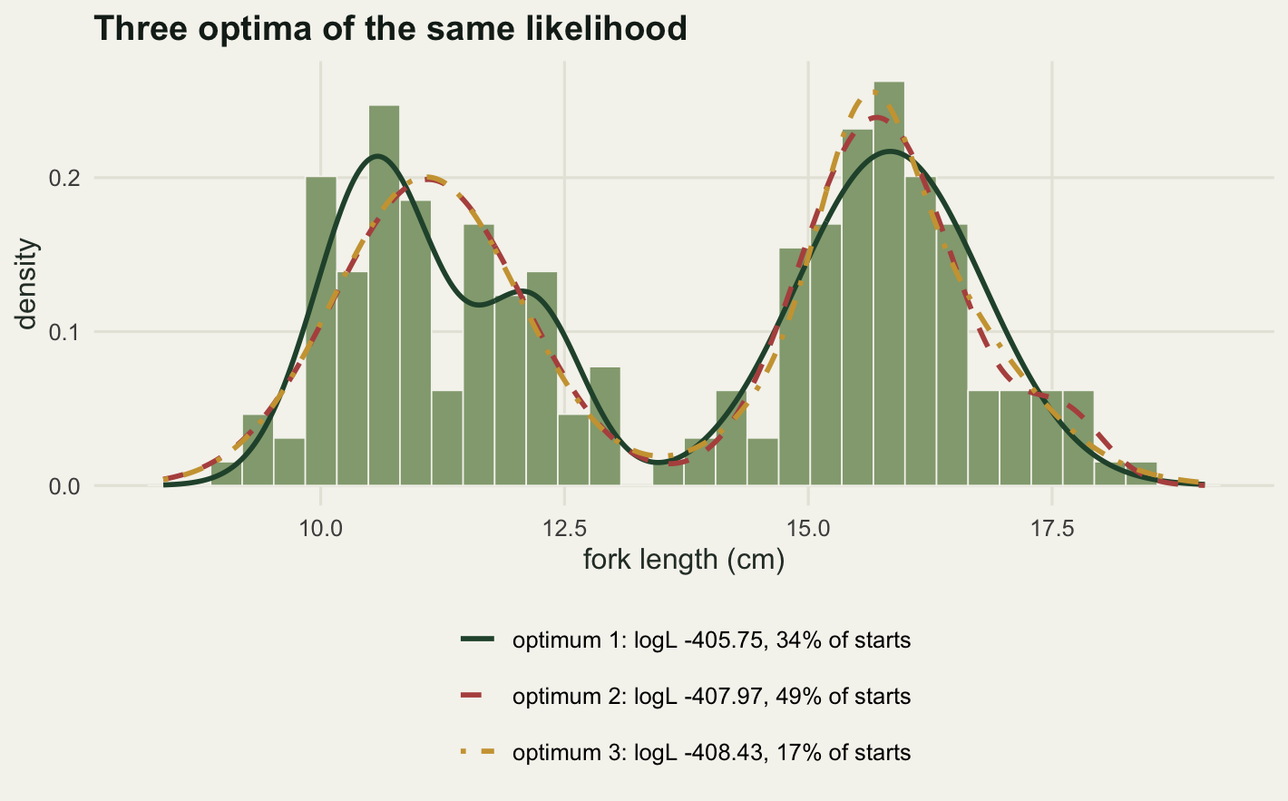
The picture explains why the plurality answer is easy to accept. The two worse curves are not obviously wrong: they track the histogram on both groups, and away from the top of the right-hand peak they are hard to tell apart. What they do not do is put a peak on the shoulder near twelve centimetres, and the whole difference of 2.2158 in log-likelihood, spread over 200 fish, comes from that one feature. A difference that small in a picture is a difference in the answer: one solution says the survey caught two young cohorts, the other one.
Check two: individual assignments are not the parameters
A mixture fit produces two quite different uncertainties at the same time. The component means can be nailed down to a few per cent while the question of which component a particular fish came from is close to a coin toss, and a sentence that starts “the two cohorts differ significantly in nitrogen signature” can quietly depend on the second while being justified by the first.
The setup is a survey with two cohorts and a second measurement on every fish, a stable nitrogen isotope ratio that tracks trophic position. The question is not about lengths at all: it is whether the older cohort feeds higher up the food web. The mixture is only there to say which fish are old.
set.seed(20260730)
mu_b <- c(11.0, 13.1); sd_b <- c(0.9, 0.9); p_b <- c(0.65, 0.35)
iso_b <- c(8.0, 9.2); iso_sd <- 0.8
n_b <- 400; reps_b <- 150
gap_true <- iso_b[2] - iso_b[1]

print(round(c(n = n_b, surveys = reps_b, mu_1 = mu_b[1], mu_2 = mu_b[2],
              sd_both = sd_b[1], w_1 = p_b[1],
              iso_1 = iso_b[1], iso_2 = iso_b[2], iso_sd = iso_sd,
              true_contrast = gap_true, separation_sd = diff(mu_b) / sd_b[1]), 4))
n surveys mu_1 mu_2 sd_both
400.0000 150.0000 11.0000 13.1000 0.9000
w_1 iso_1 iso_2 iso_sd true_contrast
0.6500 8.0000 9.2000 0.8000 1.2000
separation_sd
2.3333 Two cohorts 2.3333 standard deviations apart, the younger one holding 0.65 of the catch, 400 fish per survey and 150 surveys. The nitrogen values are drawn from the cohort means 8.0 and 9.2 with a within-cohort standard deviation of 0.8, so the true contrast to be recovered is 1.2 units, and nitrogen carries no information about length beyond what the cohort label already carries.
out_b <- matrix(NA_real_, reps_b, 8)
for (r in seq_len(reps_b)) {
  g <- sample(1:2, n_b, TRUE, p_b)
  x <- rnorm(n_b, mu_b[g], sd_b[g])
  iso <- rnorm(n_b, iso_b[g], iso_sd)
  f <- em_mix(x, 2, quantile(x, c(0.25, 0.75), names = FALSE), rep(sd(x) * 0.7, 2),
              c(0.5, 0.5), maxit = 800, tol = 1e-7, sd_floor = 0.05 * sd(x))
  o <- order(f$mu); zz <- f$z[, o]
  hard <- ifelse(zz[, 1] > 0.5, 1L, 2L)
  d_hard <- mean(iso[hard == 2L]) - mean(iso[hard == 1L])
  d_soft <- sum(zz[, 2] * iso) / sum(zz[, 2]) - sum(zz[, 1] * iso) / sum(zz[, 1])
  coefs <- solve(crossprod(zz), crossprod(zz, iso))
  out_b[r, ] <- c(f$mu[o], mean(hard == 1L), f$prop[o][1], d_hard, d_soft,
                  coefs[2] - coefs[1], mean(pmax(zz[, 1], zz[, 2])))
}
colnames(out_b) <- c("mu1", "mu2", "p_hard", "p_soft", "d_hard", "d_soft", "d_reg", "maxz")
print(round(c(se_mu_1 = sd(out_b[, "mu1"]), se_mu_2 = sd(out_b[, "mu2"]),
              se_gap = sd(out_b[, "mu2"] - out_b[, "mu1"]),
              mean_gap = mean(out_b[, "mu2"] - out_b[, "mu1"]),
              true_gap = diff(mu_b),
              relative_se_gap = sd(out_b[, "mu2"] - out_b[, "mu1"]) /
                mean(out_b[, "mu2"] - out_b[, "mu1"])), 4))
se_mu_1 se_mu_2 se_gap mean_gap true_gap
0.2071 0.3622 0.1953 2.1050 2.1000
relative_se_gap
0.0928 Take the parameter uncertainty first. Over 150 surveys the first component mean has a standard error of 0.2071 centimetres and the second 0.3622. Their difference, the quantity a growth model would use, averages 2.1050 against a truth of 2.1, with a standard error of 0.1953, which is 0.0928 of the gap itself. By the standards of field ecology the means are well estimated.
set.seed(20260731)
g1 <- sample(1:2, n_b, TRUE, p_b)
x_one <- rnorm(n_b, mu_b[g1], sd_b[g1])
f_one <- em_mix(x_one, 2, quantile(x_one, c(0.25, 0.75), names = FALSE),
                rep(sd(x_one) * 0.7, 2), c(0.5, 0.5), maxit = 800, tol = 1e-7,
                sd_floor = 0.05 * sd(x_one))
o_one <- order(f_one$mu); z_one <- f_one$z[, o_one]
maxz <- pmax(z_one[, 1], z_one[, 2])
hi_cut <- 0.95; mid_cut <- 0.90; low_cut <- 0.75
print(round(c(high_cut = hi_cut, mid_cut = mid_cut, low_cut = low_cut,
              mean_max_posterior = mean(maxz), share_above_high = mean(maxz > hi_cut),
              share_below_mid = mean(maxz < mid_cut),
              share_below_low = mean(maxz < low_cut),
              misfiled = mean(ifelse(z_one[, 1] > 0.5, 1L, 2L) != g1)), 4))
high_cut mid_cut low_cut mean_max_posterior
0.9500 0.9000 0.7500 0.8957
share_above_high share_below_mid share_below_low misfiled
0.5400 0.3700 0.1650 0.1025 Now the classification uncertainty on one survey from the same generator. The average largest membership probability is 0.8957. A share of 0.5400 of the fish are assigned with a probability above 0.95, 0.3700 sit below 0.90, and 0.1650 are close enough to a coin toss to carry almost no information. Against the labels that generated the data, 0.1025 of the fish end up in the wrong cohort.
Both statements are true of the same fit. The cohorts are separated well enough that their means are recovered to a fraction of a centimetre and badly enough that one fish in ten is misfiled, and the standard errors on the means say nothing about the second.
est_b <- out_b[, c("d_hard", "d_soft", "d_reg")]
tab_b <- data.frame(
  estimator = c("hard assignment", "posterior weighted mean", "regression on weights"),
  mean_estimate = round(colMeans(est_b), 4),
  bias = round(colMeans(est_b) - gap_true, 4),
  sd_across_surveys = round(apply(est_b, 2, sd), 4),
  rmse = round(sqrt(colMeans((est_b - gap_true)^2)), 4))
rownames(tab_b) <- NULL
print(tab_b)
estimator mean_estimate bias sd_across_surveys rmse
1 hard assignment 0.8666 -0.3334 0.1283 0.3570
2 posterior weighted mean 0.7531 -0.4469 0.1152 0.4615
3 regression on weights 1.1943 -0.0057 0.1267 0.1264print(round(c(extra_bias_of_soft = abs(tab_b$bias[2]) - abs(tab_b$bias[1]),
rmse_ratio_soft_to_regression = tab_b$rmse[2] / tab_b$rmse[3]), 4)) extra_bias_of_soft rmse_ratio_soft_to_regression
0.1135 3.6511 print(round(c(w1_true = p_b[1], w1_hard = mean(out_b[, "p_hard"]),
w1_soft = mean(out_b[, "p_soft"]),
bias_hard = mean(out_b[, "p_hard"]) - p_b[1],
bias_soft = mean(out_b[, "p_soft"]) - p_b[1]), 4)) w1_true w1_hard w1_soft bias_hard bias_soft
0.6500 0.6389 0.6235 -0.0111 -0.0265 Three ways to get the nitrogen contrast out of the same fit. Hard assignment sends every fish to its most probable cohort and takes two ordinary means. Posterior weighting takes two weighted means with the membership probabilities as weights, which is the advice in every tutorial including, until this measurement was run, the plan for this one. Regression takes the two probability columns as predictors and fits nitrogen against them with no intercept.
Hard assignment gives 0.8666 against a truth of 1.2, a bias of -0.3334. Posterior weighting gives 0.7531, a bias of -0.4469. The recommended estimator is 0.1135 further from the truth than the one it replaces, with a root mean squared error of 0.4615 against 0.3570. Both shrink the contrast towards zero and the softer one shrinks it harder.
The reason shows up in what each weight does to a fish that belongs to the older cohort but looks young. Under posterior weighting that fish contributes its full membership probability to the young mean, and so does every other older fish, including those whose probability of being young is a twentieth: small contributions, numerous, all pulling the same way. Under hard assignment every fish with a young probability below one half contributes nothing, which throws away that accumulated leakage in exchange for occasionally sending one fish entirely to the wrong side. On these numbers the trade is worth making.
The third estimator is not a compromise, it is the correct one. The expected nitrogen value of a fish, given its length, is its young membership probability times the young cohort mean plus its old membership probability times the old cohort mean: a linear model in the two cohort means with the probabilities as the design matrix, so least squares recovers them. The estimate is 1.1943, a bias of -0.0057 and a root mean squared error of 0.1264, which is 3.6511 times smaller than the weighted mean it replaces, for one line of code: solve(crossprod(z), crossprod(z, y)).
The mixing weight is the one quantity where the difference is small. The true young share is 0.65; counting hard assignments gives 0.6389 and reading the fitted weight gives 0.6235, biases of -0.0111 and -0.0265. Both are small next to the sampling variation, which is why the hard-versus-soft argument so often goes unresolved: on the quantity people usually check, it does not matter. It matters on the quantity they do not check.
lv_b <- tab_b$estimator
long_b <- data.frame(v = as.numeric(est_b),
                     series = factor(rep(lv_b, each = reps_b), levels = lv_b))
ggplot(long_b, aes(v, colour = series, fill = series)) +
  geom_density(alpha = 0.25, linewidth = 0.9, bw = 0.05) +
  geom_vline(xintercept = gap_true, colour = te_pal$ink, linetype = 2, linewidth = 0.7) +
  annotate("text", x = gap_true, y = 0, label = "truth", hjust = -0.15, vjust = -0.6,
           size = 3.5, colour = te_pal$ink) +
  scale_colour_manual(values = c(te_pal$clay, te_pal$gold, te_pal$green), name = NULL) +
  scale_fill_manual(values = c(te_pal$clay, te_pal$gold, te_pal$green), name = NULL) +
  guides(colour = guide_legend(nrow = 2), fill = guide_legend(nrow = 2)) +
  labs(title = "Three ways to read a class contrast off one fit",
       x = "estimated nitrogen difference between cohorts",
       y = "density over 150 surveys") +
  theme_te()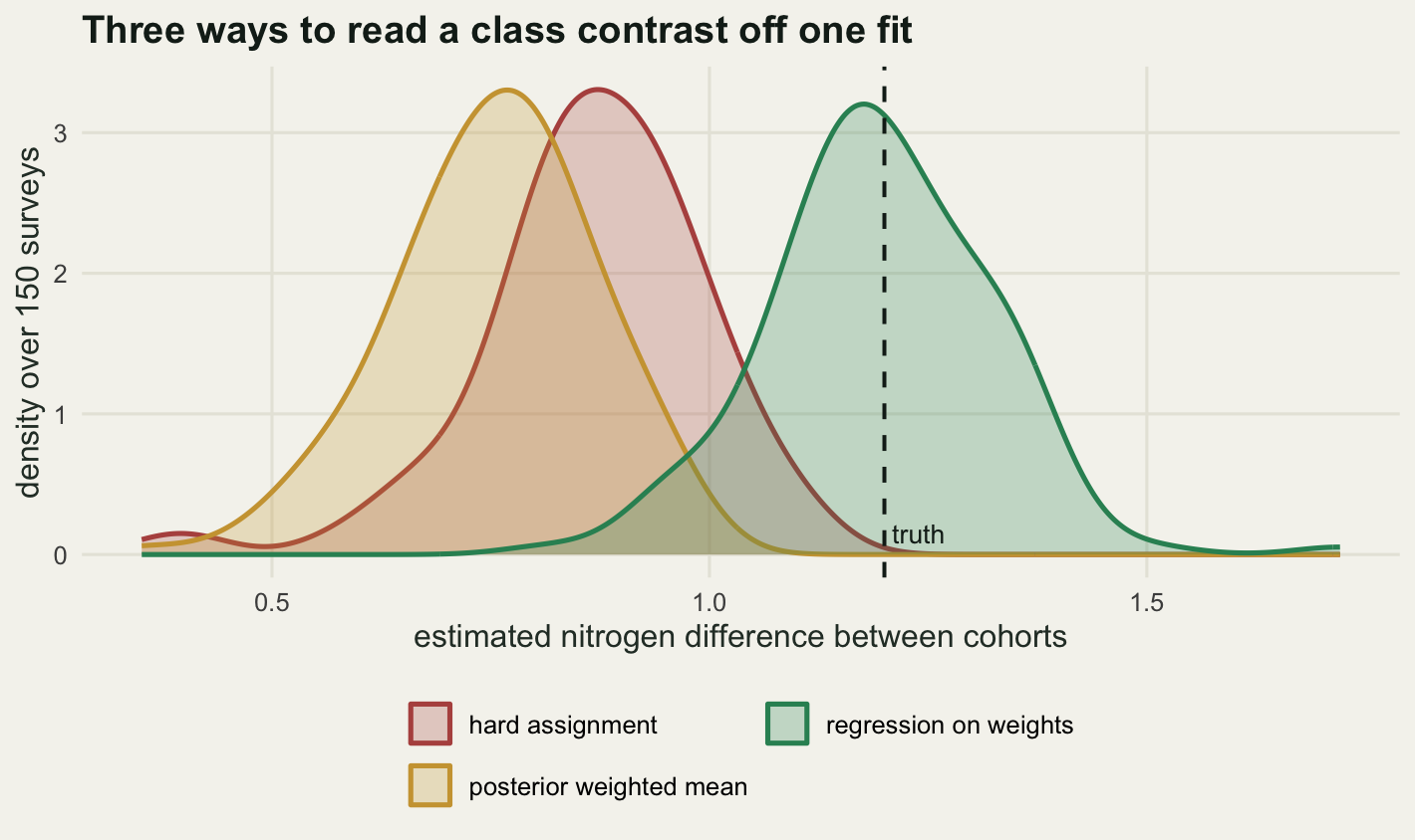
The three distributions have almost the same width, which is the useful part of the picture: the difference between these estimators is not about precision. All three would give a similar confidence interval, all three would be “significant”, and two would be significantly wrong. A bootstrap over the fish resamples the same bias every time and reports it as certainty.
Check three: the likelihood has no maximum
With unequal variances allowed, the likelihood of a normal mixture is unbounded. Put one component exactly on one observation and let its standard deviation go to zero: that observation’s density goes to infinity, the rest are still covered by the other components, and the likelihood grows without limit. There is no maximum to find. Every finite answer EM returns is a local optimum in the interior, and the supremum is a solution saying one fish is a cohort of one. This is a property of the model, not a numerical quirk, and the standard responses all change the model or the estimator rather than the code.
spread_start <- function(x, K) {
  list(mu = sample(x, K), sdev = sd(x) * runif(K, 0.02, 1.2), prop = rep(1 / K, K))
}
mu_c <- c(11.0, 13.0); sd_c <- c(1.0, 0.4); p_c <- c(0.5, 0.5)
hard_floor <- 1e-8
set.seed(20260801)
n_grid <- c(20, 40, 80, 160); sets_c <- 40; starts_c <- 8
print(round(c(datasets_per_n = sets_c, starts_per_dataset = starts_c,
              mu_1 = mu_c[1], mu_2 = mu_c[2], sd_1 = sd_c[1], sd_2 = sd_c[2],
              smallest_start_sd_factor = 0.02, degenerate_cut = 0.01), 4))
datasets_per_n starts_per_dataset mu_1
40.00 8.00 11.00
mu_2 sd_1 sd_2
13.00 1.00 0.40
smallest_start_sd_factor degenerate_cut
0.02 0.01 print(signif(c(numerical_floor = hard_floor), 1))numerical_floor
1e-08 tab_c <- NULL
for (nn in n_grid) {
hit <- 0; best_hit <- 0
for (d in seq_len(sets_c)) {
x <- rmix(nn, mu_c, sd_c, p_c); sx <- sd(x)
lls <- numeric(starts_c); bad <- logical(starts_c)
for (s in seq_len(starts_c)) {
st <- spread_start(x, 2)
f <- em_mix(x, 2, st$mu, st$sdev, st$prop, maxit = 400, tol = 1e-9,
sd_floor = hard_floor)
lls[s] <- f$loglik; bad[s] <- min(f$sd) < 0.01 * sx # collapsed onto a point
}
hit <- hit + sum(bad); best_hit <- best_hit + bad[which.max(lls)]
}
tab_c <- rbind(tab_c, data.frame(n = nn,
per_start = round(hit / (sets_c * starts_c), 4),
per_dataset = round(best_hit / sets_c, 4)))
}
print(tab_c) n per_start per_dataset
1 20 0.0312 0.175
2 40 0.0375 0.125
3 80 0.0281 0.000
4 160 0.0281 0.000The truth here has genuinely unequal spreads, 1.0 and 0.4 centimetres, so an equal-variance model is wrong and the unbounded likelihood is not avoidable by assumption. spread_start differs from the earlier starter in one respect: it allows a starting standard deviation as small as 0.02 times the overall spread. That is what a genuinely random start looks like, and a starter that only proposes wide components never discovers this problem exists. A solution counts as degenerate when its smaller standard deviation falls below 0.01 of the overall spread; the floor at 1e-08 is numerical only.
Two rates are reported per sample size, and they are not the same measurement. The per-start rate, the share of EM runs that collapse onto a point, is 0.0312 at n = 20 and 0.0281 at n = 160. The per-dataset rate, the share of datasets on which the best of 8 starts is degenerate, falls from 0.1750 to 0.1250 to 0.0000 and then to 0.0000.
The two rates count different things. The per-start rate has EM runs in its denominator, the per-dataset rate has datasets, and a dataset only counts as degenerate when the best of its starts is. Whether the degenerate solution wins is a separate question: its advantage is a fixed bonus from the one observation it sits on, while the sensible solution’s advantage grows with every observation it explains properly.
set.seed(20260805)
x_c <- rmix(25, mu_c, sd_c, p_c); sx_c <- sd(x_c)
ll_c <- numeric(40); min_c <- numeric(40); fit_c <- vector("list", 40)
for (s in seq_len(40)) {
  st <- spread_start(x_c, 2)
  f <- em_mix(x_c, 2, st$mu, st$sdev, st$prop, maxit = 600, tol = 1e-10,
              sd_floor = hard_floor)
  ll_c[s] <- f$loglik; min_c[s] <- min(f$sd); fit_c[[s]] <- f
}

bad_c <- which(min_c < 0.01 * sx_c); ok_c <- which(min_c >= 0.01 * sx_c)
jb <- bad_c[which.max(ll_c[bad_c])]; jo <- ok_c[which.max(ll_c[ok_c])]
print(round(c(sample_size = 25, starts = 40, degenerate_starts = length(bad_c),
              logLik_degenerate = ll_c[jb], logLik_sensible = ll_c[jo],
              logLik_advantage = ll_c[jb] - ll_c[jo],
              weight_of_spike = min(fit_c[[jb]]$prop)), 4))
sample_size starts degenerate_starts logLik_degenerate
25.0000 40.0000 1.0000 -22.6771
logLik_sensible logLik_advantage weight_of_spike
-29.6832 7.0062 0.0400 One worked example makes the scale concrete. Twenty-five fish, forty random starts, 1 of them collapsed. The collapsed solution reaches a log-likelihood of -22.6771 against -29.6832 for the best sensible one, ahead by 7.0062 units, which by AIC or a likelihood ratio wins by a distance. Its weight is 0.0400, which on twenty-five fish is exactly one fish. A selection procedure that trusts the likelihood will choose the model in which one fish is a cohort.
set.seed(20260803)
n_r <- 40; sets_r <- 100; starts_r <- 4
best_of <- function(x, ...) {
  bf <- NULL
  for (s in seq_len(starts_r)) {
    st <- spread_start(x, 2)
    f <- em_mix(x, 2, st$mu, st$sdev, st$prop, maxit = 400, tol = 1e-9, ...)
    if (is.null(bf) || f$loglik > bf$loglik) bf <- f
  }
  bf
}
pen_an <- 1 / sqrt(n_r)
acc <- array(NA_real_, c(sets_r, 4, 5))
for (d in seq_len(sets_r)) {
  x <- rmix(n_r, mu_c, sd_c, p_c); sx <- sd(x)
  fits <- list(best_of(x, sd_floor = hard_floor),   # no repair
               best_of(x, sd_floor = 0.1 * sx),
               best_of(x, sd_floor = hard_floor, equal_var = TRUE),
               best_of(x, sd_floor = hard_floor, pen_a = pen_an))
  for (m in 1:4) {
    f <- fits[[m]]; o <- order(f$mu)
    acc[d, m, ] <- c(f$mu[o], f$sd[o], min(f$sd) < 0.01 * sx)
  }
}


rmse_of <- function(m, target) round(sqrt(colMeans((m - target)^2)), 4)
tab_r <- data.frame(
  repair = c("none", "variance floor", "equal variances", "variance penalty"),
  degenerate = round(colMeans(acc[, , 5]), 4),
  rmse_mu_1 = rmse_of(acc[, , 1], mu_c[1]), rmse_mu_2 = rmse_of(acc[, , 2], mu_c[2]),
  mean_sd_1 = round(colMeans(acc[, , 3]), 4), mean_sd_2 = round(colMeans(acc[, , 4]), 4),
  rmse_sd_2 = rmse_of(acc[, , 4], sd_c[2]))
print(round(c(repair_n = n_r, repair_datasets = sets_r, repair_starts = starts_r,
              penalty_weight = pen_an,
              percent_degenerate_no_repair = 100 * mean(acc[, 1, 5])), 4))
repair_n repair_datasets
40.0000 100.0000
repair_starts penalty_weight
4.0000 0.1581
percent_degenerate_no_repair
5.0000 print(tab_r) repair degenerate rmse_mu_1 rmse_mu_2 mean_sd_1 mean_sd_2 rmse_sd_2
1 none 0.05 0.5878 0.2659 0.8571 0.3924 0.1935
2 variance floor 0.00 0.4486 0.1701 0.8830 0.3757 0.1414
3 equal variances 0.00 0.5779 0.2743 0.6231 0.6231 0.2474
4 variance penalty 0.00 0.3851 0.1435 0.8487 0.4526 0.1093Three repairs, measured on 100 datasets of 40 fish each, 4 starts per dataset and the best kept. The variance floor forbids any standard deviation below a tenth of the overall spread. The equal-variance constraint gives every component the same standard deviation, which removes the degeneracy by construction because a shared variance cannot collapse onto one point. The penalty punishes small variances with weight 0.1581, one over the square root of the sample size, pulling each variance update towards the overall variance of the data.
Doing nothing gives a degenerate best solution on 5 per cent of the datasets, and all three repairs remove that completely. What they cost is the interesting part, because the truth here has unequal variances and two of the three repairs are lies about it.
The equal-variance constraint is the one that fails. Its root mean squared error on the broad component’s mean is 0.5779 against 0.5878 for no repair at all, and on the narrow component’s mean 0.2743 against 0.2659. On the means it is a wash. On the spreads it is worse, returning an average standard deviation of 0.6231 for both components when the truth is 1.0 and 0.4, so the fitted model cannot say that older fish are more variable in length than young ones, which is often the result of interest.
The variance floor does better than expected, 0.4486 and 0.1701 on the two means, both better than no repair. The penalty does better still, 0.3851 and 0.1435, and it improves the narrow component’s spread most, with a root mean squared error of 0.1093 against 0.1414 for the floor and 0.1935 for no repair. Its average estimate of that standard deviation is 0.4526 against a truth of 0.4, slightly too large, which is what a penalty towards the overall spread should do.
lv_r <- c("mean of the broad component", "mean of the narrow component",
          "sd of the narrow component")
long_r <- data.frame(repair = factor(rep(tab_r$repair, 3), levels = rev(tab_r$repair)),
                     v = c(tab_r$rmse_mu_1, tab_r$rmse_mu_2, tab_r$rmse_sd_2),
                     series = factor(rep(lv_r, each = 4), levels = lv_r))
ggplot(long_r, aes(v, repair, colour = series, shape = series)) +
  geom_point(size = 3.4) +
  scale_colour_manual(values = c(te_pal$forest, te_pal$gold, te_pal$clay), name = NULL) +
  scale_shape_manual(values = c(16, 17, 15), name = NULL) +
  guides(colour = guide_legend(nrow = 2), shape = guide_legend(nrow = 2)) +
  labs(title = "What each repair costs",
       x = "root mean squared error (cm)", y = NULL) +
  theme_te() +
  theme(plot.margin = margin(6, 16, 6, 6))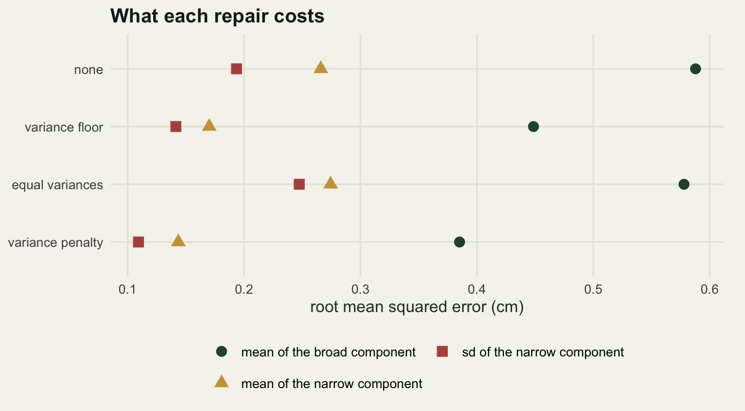
The ordering in the picture is the practical advice. If the components really do differ in spread, and in a length frequency they almost always do, the penalty costs least and buys most. The floor is a reasonable second, with the caveat that its value is arbitrary and the answer depends on it. The equal-variance model is worth fitting when you believe it, not as a way of making a warning go away. The floor imposed back in check one was not decoration either: without it, some of the optima counted there would have been spikes rather than genuine local maxima, so constraints on the variance change which optima exist and the two checks have to be run in that order.
Check four: does the fit describe the data
The first three checks are about the fitting. The fourth is about the model. Simulate new samples from the fitted mixture, compute a summary on each, and see where the real sample falls in that reference distribution. The summary has to be something the likelihood is not already fitting, because a summary it fits will match by construction and the check will pass whatever is wrong.
n_modes <- function(x, bw) {
  d <- density(x, bw = bw, n = 512)$y
  sum(d[2:511] > d[1:510] & d[2:511] > d[3:512])
}
pmix <- function(q, mu, sdev, prop) {
  out <- numeric(length(q))
  for (k in seq_along(mu)) out <- out + prop[k] * pnorm(q, mu[k], sdev[k])
  out
}
ks_gap <- function(x, f) {
  s <- sort(x); m <- length(s); Fh <- pmix(s, f$mu, f$sd, f$prop)
  max(pmax(seq_len(m) / m - Fh, Fh - (seq_len(m) - 1) / m))
}
fit_k2 <- function(x, tries = 4) {
  bf <- NULL
  for (s in seq_len(tries)) {
    st <- rand_start(x, 2, 0.3, 1.2)
    f <- em_mix(x, 2, st$mu, st$sdev, st$prop, maxit = 600, tol = 1e-8,
                sd_floor = 0.05 * sd(x))
    if (is.null(bf) || f$loglik > bf$loglik) bf <- f
  }
  bf
}
Three summaries. The sample variance is a moment, and a two-component mixture can match the first two moments of almost anything, so it is expected to pass no matter what. The number of modes of a kernel density estimate is the textbook choice, because the number of bumps is exactly what a wrong number of components should get wrong; it uses a bandwidth fixed from the real sample and reused unchanged on every simulated one. The largest gap between the empirical and the fitted distribution function is the shape summary.
set.seed(20260806)
n_d <- 300; B_d <- 150
mu_ok <- c(11.0, 14.0); mu_bad <- c(11.0, 15.0, 19.0); sd_d <- 0.8
x_ok <- rmix(n_d, mu_ok, rep(sd_d, 2), rep(0.5, 2))
x_bad <- rmix(n_d, mu_bad, rep(sd_d, 3), rep(1 / 3, 3))
print(round(c(n = n_d, replicates = B_d, sd_all = sd_d,
              ok_1 = mu_ok[1], ok_2 = mu_ok[2],
              bad_1 = mu_bad[1], bad_2 = mu_bad[2], bad_3 = mu_bad[3]), 4))
n replicates sd_all ok_1 ok_2 bad_1 bad_2
300.0 150.0 0.8 11.0 14.0 11.0 15.0
bad_3
19.0 ppc <- function(x) {
f <- fit_k2(x); bw <- bw.nrd0(x)
obs <- c(variance = var(x), modes = n_modes(x, bw), ks = ks_gap(x, f))
sim <- matrix(NA_real_, B_d, 4)
for (b in seq_len(B_d)) {
xs <- rmix(n_d, f$mu, f$sd, f$prop); fb <- fit_k2(xs, 2)
sim[b, ] <- c(var(xs), n_modes(xs, bw), ks_gap(xs, f), ks_gap(xs, fb))
}
p_var <- min(1, 2 * min(mean(sim[, 1] >= obs[1]), mean(sim[, 1] <= obs[1])))
list(fit = f, bw = bw, obs = obs, sim = sim,
p = c(variance = p_var, modes = mean(sim[, 2] >= obs[2]),
ks_plugin = mean(sim[, 3] >= obs[3]), ks_refit = mean(sim[, 4] >= obs[3])))
}
r_ok <- ppc(x_ok)
r_bad <- ppc(x_bad)
tab_d <- data.frame(summary_used = c("variance", "number of modes", "largest CDF gap"),
observed_correct = round(r_ok$obs, 4), p_correct = round(r_ok$p[1:3], 4),
observed_wrong = round(r_bad$obs, 4), p_wrong = round(r_bad$p[1:3], 4))
rownames(tab_d) <- NULL
print(tab_d) summary_used observed_correct p_correct observed_wrong p_wrong
1 variance 3.0208 0.8933 11.4712 0.9600
2 number of modes 2.0000 1.0000 3.0000 0.0333
3 largest CDF gap 0.0187 1.0000 0.1022 0.0000print(round(c(bw_correct = r_ok$bw, bw_wrong = r_bad$bw,
wrong_fit_mu_1 = sort(r_bad$fit$mu)[1],
wrong_fit_mu_2 = sort(r_bad$fit$mu)[2],
p_resolution = 1 / B_d,
sims_reaching_three_modes = sum(r_bad$sim[, 2] >= 3)), 4)) bw_correct bw_wrong wrong_fit_mu_1
0.4999 0.9741 13.2705
wrong_fit_mu_2 p_resolution sims_reaching_three_modes
19.0472 0.0067 5.0000 Two datasets, both fitted with two components. The first really has two cohorts at 11.0 and 14.0 centimetres, so the model is right. The second has three at 11.0, 15.0 and 19.0, so the model is a whole cohort short. Each check uses 150 simulated samples of 300 fish, which puts the finest resolvable p-value at 0.0067.
On the correct fit every summary passes, as it should: 0.8933 for the variance, 1.0000 for the number of modes and 1.0000 for the largest gap. The last two are exactly 1, which is a warning in itself and is taken up below.
On the wrong fit the three disagree completely. The variance gives 0.9600: the model is missing an entire cohort and the moment check does not notice, because the fit spent its freedom on matching the spread. The fitted means are 13.2705 and 19.0472 centimetres, one broad component swallowing the two lower cohorts and a narrower one on the top, and the variance comes out right even though the shape does not.
The mode count gives 0.0333. The real sample has 3 modes at the chosen bandwidth of 0.9741, and 5 of the 150 simulated samples reached three modes too, enough to keep the p-value off the floor. The summary that was supposed to be decisive only just clears the conventional threshold, because a two-component mixture throws a spurious third bump often enough to blunt the test, and the bandwidth that controls how often is a free choice made by the analyst.
The largest gap between the empirical and fitted distribution functions gives 0.0000: not one of the 150 simulated samples came close to the real one. The summary expected to be the dull technical option is the one that answers the question.
sl_d <- c("variance", "number of modes", "largest CDF gap")
pan_lv <- c(paste0("correct fit: ", sl_d), paste0("wrong fit: ", sl_d))
mk_d <- function(r, lab) do.call(rbind, lapply(1:3, function(j)
  data.frame(value = r$sim[, j], panel = paste0(lab, ": ", sl_d[j]))))
sims_d <- rbind(mk_d(r_ok, "correct fit"), mk_d(r_bad, "wrong fit"))
sims_d$panel <- factor(sims_d$panel, levels = pan_lv)
obs_d <- data.frame(value = c(as.numeric(r_ok$obs), as.numeric(r_bad$obs)),
                    panel = factor(pan_lv, levels = pan_lv), series = "real sample")
ggplot(sims_d, aes(value)) +
  geom_histogram(bins = 18, fill = te_pal$sage, colour = te_pal$paper, linewidth = 0.25) +
  geom_vline(data = obs_d, aes(xintercept = value, colour = series),
             linetype = 2, linewidth = 0.9) +
  facet_wrap(~ panel, scales = "free", ncol = 3) +
  scale_colour_manual(values = te_pal$clay, name = NULL) +
  labs(title = "Reference distributions for three summaries",
       x = "value of the summary", y = "count over 150 simulated surveys") +
  theme_te() +
  theme(strip.text = element_text(colour = "#2c3a31", size = 9.5),
        plot.margin = margin(6, 14, 6, 6))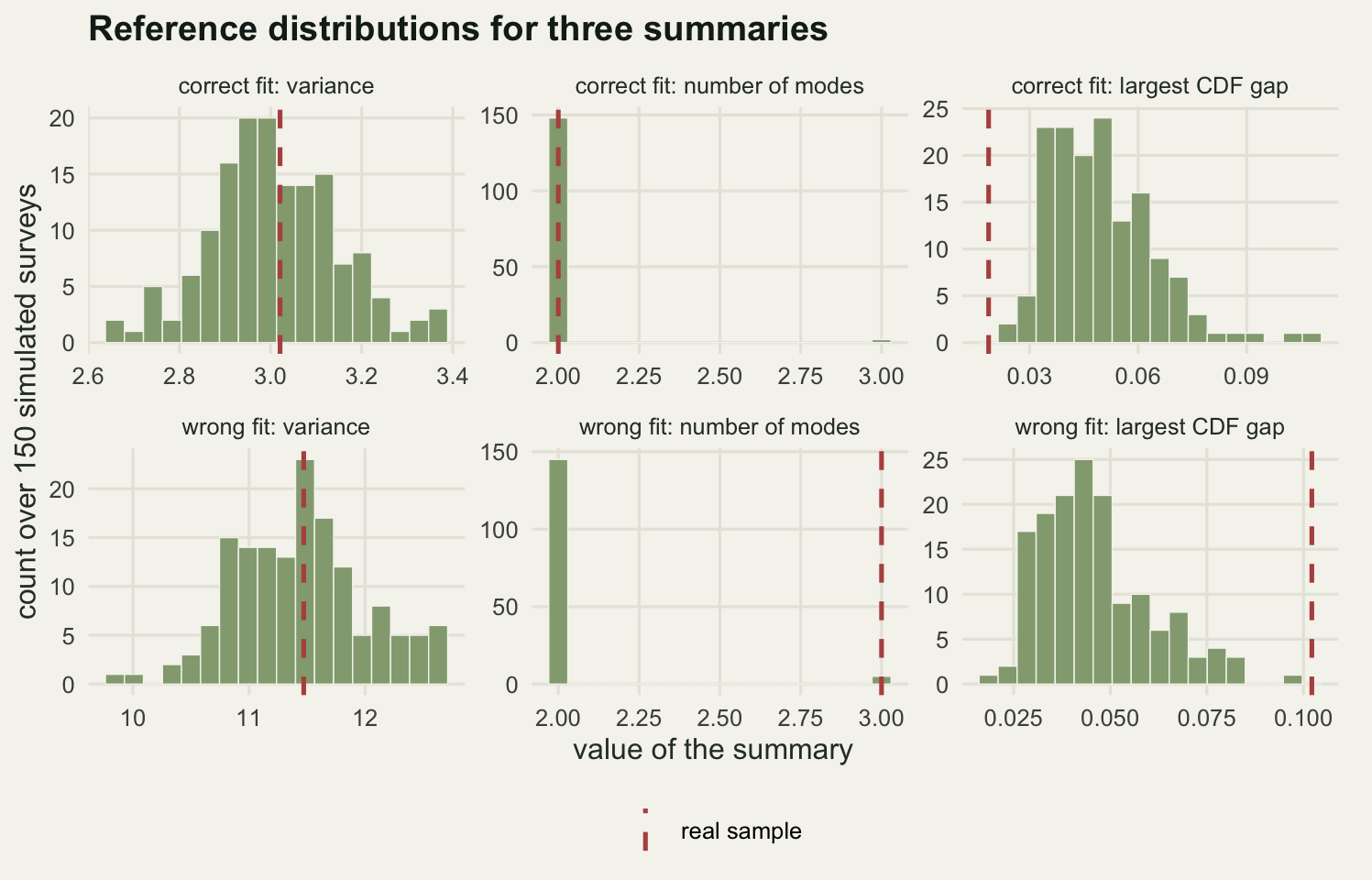
The two p-values of exactly 1 in the top row need explaining, and they need separate explanations. The mode count sits at the bottom of its own reference distribution: the real sample has 2 modes, 148 of the 150 simulated samples have the same count and none has fewer, so a p-value that counts ties comes out at 1 by construction. The only direction that summary can flag is upwards, and the real sample is already at the floor. The largest CDF gap is the one that exposes a real defect in the check as written. The reference samples came from the fitted parameters, but those parameters were tuned to the real sample, so the real sample fits them better than any fresh sample from them ever will. That check is conservative: it fails to reject models it should reject.
print(round(c(mean_gap_plugin = mean(r_ok$sim[, 3]),
              mean_gap_refit = mean(r_ok$sim[, 4]),
              width_ratio = mean(r_ok$sim[, 3]) / mean(r_ok$sim[, 4]),
              p_refit_correct = r_ok$p["ks_refit"],
              p_refit_wrong = r_bad$p["ks_refit"]), 4))
mean_gap_plugin mean_gap_refit width_ratio
0.0498 0.0269 1.8513
p_refit_correct.ks_refit p_refit_wrong.ks_refit
0.9800 0.0000 The loop above already measured the size of the defect: alongside each simulated sample’s gap against the fixed fitted parameters, it recorded the gap against a mixture refitted to that sample. On the correct fit the plug-in reference gaps average 0.0498 and the refitted ones 0.0269, so the reference distribution is 1.8513 times too wide, which is where the p-value of 1 came from.
Refitting each simulated sample repairs it: the correct fit then gives 0.9800, no longer pinned at the ceiling, and the wrong fit 0.0000. The conclusion does not change here, but the calibration costs one extra model fit per simulated sample, and on a model that takes minutes rather than milliseconds that is the difference between doing the check and skipping it.
What to take away
Four checks, and three of them came back against the plan. Running many starts found 3 optima, and the one that most starts reached was not the best: 49.17 per cent of runs landed on a solution worse by 2.2158 in log-likelihood than the one 34.17 per cent found. The recommended way to carry classification uncertainty into a downstream contrast, weighting by the membership probabilities, was more biased than the hard assignment it replaces, -0.4469 against -0.3334, and what works is a regression of the second variable on the two probability columns, bias -0.0057. The equal-variance constraint stopped the likelihood degenerating, as advertised, and gave back nothing on the component means, 0.2743 against 0.2659 for no repair at all, while forcing both spreads to 0.6231 when the truth was 1.0 and 0.4. The fourth check kept its verdict but swapped its summaries round: the mode count, the summary everyone reaches for, only just cleared the threshold at 0.0333 on a model missing an entire cohort, while the plain distribution function comparison, written in as the dull technical option, gave 0.0000.
The honest limit is that every number here comes from a simulation in which the components are exactly normal and the model is correct except where it was deliberately broken, and the first and fourth checks each rest on a single simulated dataset, so the count of optima and the individual p-values are one draw rather than an expectation. Real length frequencies are skewed within cohort, growth overlaps the cohorts more than these settings do, and gill nets select on size, so a mixture fitted to a real catch is already misspecified before any of these checks is run. The directions will hold; the sizes are a rough scale.
What survives is a short list, and none of it needs more data. Run the fit from many random starts and keep the best rather than the commonest. Sort the components before averaging anything across runs, and check that sorting removed the differences rather than assuming it did. Report the distribution of the largest membership probability next to the standard errors on the means, because they answer different questions. If a downstream quantity depends on the classification, regress it on the probability columns rather than averaging with them. Penalise the variances rather than equating them. And when a predictive check passes, look at which summary passed, because a moment will pass for a model missing a whole cohort.
References
McLachlan GJ, Peel D 2000 Finite Mixture Models (ISBN 978-0-471-00626-8)
Redner RA, Walker HF 1984 SIAM Review 26(2):195-239 (10.1137/1026034)
Stephens M 2000 Journal of the Royal Statistical Society Series B 62(4):795-809 (10.1111/1467-9868.00265)
Celeux G, Hurn M, Robert CP 2000 Journal of the American Statistical Association 95(451):957-970 (10.1080/01621459.2000.10474285)
Hennig C 2004 Annals of Statistics 32(4):1313-1340 (10.1214/009053604000000571)
Scrucca L, Fop M, Murphy TB, Raftery AE 2016 The R Journal 8(1):289-317 (10.32614/RJ-2016-021)
Conn PB, Johnson DS, Williams PJ, Melin SR, Hooten MB 2018 Ecological Monographs 88(4):526-542 (10.1002/ecm.1314)