library(ggplot2)

te_pal <- list(forest = "#275139", green = "#2f8f63", sage = "#93a87f",
               clay = "#b5534e", gold = "#cda23f", line = "#dad9ca",
               ink = "#16241d", paper = "#f5f4ee")

theme_te <- function() {
  theme_minimal(base_size = 12) +
    theme(panel.grid.minor = element_blank(),
          panel.grid.major = element_line(colour = "#e7e6dc"),
          plot.background = element_rect(fill = "#f5f4ee", colour = NA),
          panel.background = element_rect(fill = "#f5f4ee", colour = NA),
          plot.title = element_text(face = "bold", colour = te_pal$ink),
          axis.title = element_text(colour = "#2c3a31"),
          legend.position = "bottom")
}

comp_col <- c(te_pal$forest, te_pal$green, te_pal$gold, te_pal$clay)Fitting a mixture of normals in R
R
mixture models
EM
ecology tutorial
Separate fish age classes in a length-frequency sample with a finite mixture of normals: the EM algorithm written by hand in base R, and where it breaks down.
The gill net came up at first light with about two thousand fish in it, and by the time the sun was properly up the whole catch had been measured, one fish at a time, onto a plastic board with a ruler screwed to it. Fork length to the nearest millimetre, called out and written down. Nothing else was recorded: no otoliths, no scales, no ageing at all, because ageing two thousand fish is a winter of microscope work and this was a one-day survey.
Back at the desk, the histogram of those lengths is not a smooth hump. There is a sharp spike near twenty centimetres, a second clear bump near thirty, and then the right-hand side spreads out into a long shoulder carrying one much fainter rise and nothing after it. Anyone who works on fish knows what the bumps are. Fish born in the same year grow together, and in a species that spawns once a year the youngest cohorts sit in separate places on the length axis. The spike is the one-year-olds. The second bump is the two-year-olds. The faint rise is the three-year-olds, barely holding on, and the featureless part beyond it is the oldest class, which has no bump of its own because growth slows down with age while variation in length within a cohort keeps increasing.
The question is whether the histogram can be taken apart again. If each age class contributes a normal distribution of lengths, then the histogram is a weighted sum of normal curves, and the weights are the age composition of the catch. That object is a finite mixture of normals, and there is a fifty-year-old algorithm that fits one: expectation maximisation, which alternates between guessing which fish belong to which class and re-estimating the class parameters from those guesses. It fits in about twenty lines of base R and it needs no packages at all.
This post builds the whole thing from scratch on simulated data where the answer is known, and then spends most of its length on the parts that go wrong. EM converges to whatever local maximum it started nearest to, and forty random starts on these data end up in three clearly separated places, most of them well short of the best. The likelihood of an unrestricted normal mixture has no maximum at all: it can be driven to infinity by shrinking one component onto a single fish. And the classification that EM hands back is soft, a probability per fish per class, which is not what a downstream stock assessment usually wants.
This blog has fitted two-component mixtures several times already, but always inside another model where the components were known things: a structural zero and a Poisson count in zero-inflated count models, a detection and a false positive in an occupancy model, two source populations in an ancestry model. In every one of those the components had names before the data arrived. Here the mixture is the whole model and the components are unknown: nothing in the data says which fish is which age, and the algorithm has to invent the classes as well as estimate them. That is a different and much less comfortable problem, and the difference is what this post is about.
A length sample with the ages taken out
The simulated survey has four age classes. Mean length at age follows a von Bertalanffy curve with an asymptotic length of 62 cm, a growth coefficient of 0.28 per year and a length-zero age of -0.35 years, which is a perfectly ordinary set of numbers for a medium-sized freshwater fish. Length within an age class is normal with a standard deviation equal to 0.07 of the mean, so the older, longer classes are also the more variable ones. Abundance declines geometrically with age under a constant total instantaneous mortality of 0.35 per year.
Those three choices between them decide how hard the problem is. The von Bertalanffy curve makes successive mean lengths get closer together as age increases; the proportional standard deviation makes the older components wider; the mortality makes them rarer. All three push in the same direction, and they are why the right side of a real length-frequency histogram is a shoulder rather than a row of bumps.
set.seed(20260729)

linf <- 62; k_vb <- 0.28; t_zero <- -0.35
cv_len <- 0.07; z_mort <- 0.35
n_fish <- 2000; n_age <- 4

age_class <- 1:n_age
mu_true <- linf * (1 - exp(-k_vb * (age_class - t_zero)))
sd_true <- cv_len * mu_true
p_true <- exp(-z_mort * age_class)
p_true <- p_true / sum(p_true)

true_age <- sample(age_class, n_fish, replace = TRUE, prob = p_true)
len <- rnorm(n_fish, mu_true[true_age], sd_true[true_age])

print(round(c(linf = linf, k_vb = k_vb, t_zero = t_zero,
              cv_len = cv_len, z_mort = z_mort), 3))
linf k_vb t_zero cv_len z_mort
62.00 0.28 -0.35 0.07 0.35 print(round(rbind(mean_length = mu_true, sd_length = sd_true,
proportion = p_true,
n_in_sample = tabulate(true_age, n_age)), 3)) [,1] [,2] [,3] [,4]
mean_length 19.516 29.891 37.733 43.659
sd_length 1.366 2.092 2.641 3.056
proportion 0.392 0.276 0.195 0.137
n_in_sample 791.000 560.000 370.000 279.000gap <- diff(mu_true) / ((sd_true[-1] + sd_true[-n_age]) / 2)
print(round(c(gap_1_2 = gap[1], gap_2_3 = gap[2], gap_3_4 = gap[3],
n_fish = n_fish, n_age = n_age), 2))gap_1_2 gap_2_3 gap_3_4 n_fish n_age
6.00 3.31 2.08 2000.00 4.00 The simulated truth is 19.516, 29.891, 37.733 and 43.659 cm for the four mean lengths, with standard deviations of 1.366 to 3.056 cm and proportions running from 0.392 down to 0.137. The realised sample contains 791 one-year-olds and only 279 four-year-olds out of 2000 fish.
The last three numbers in the second block are the ones that matter. They are the distances between neighbouring means expressed in units of the average standard deviation of the two components: 6 for the first pair, 3.31 for the second and 2.08 for the third. A separation of six standard deviations means two components that barely touch. A separation of 2.08 means two curves whose bulk overlaps heavily, and a rule of thumb that has been around since Hasselblad’s 1966 paper is that anything below about two is very hard to resolve at all. The third and fourth age classes in this survey sit right on that line, and everything difficult in the rest of the post happens there.
The EM algorithm in twenty lines
The model says each fish has a hidden label \(z_i\) taking one of \(K\) values, that \(P(z_i = k) = \pi_k\), and that given the label the length is normal with mean \(\mu_k\) and standard deviation \(\sigma_k\). The likelihood of one fish is the sum over the labels it might have had, and the log-likelihood of the sample is
\[\ell(\theta) = \sum_{i=1}^{n} \log \sum_{k=1}^{K} \pi_k \, \phi(x_i \mid \mu_k, \sigma_k).\]
That log of a sum is the whole problem. It does not factorise, so there is no closed form for the estimates. EM gets around it by pretending, for the length of one iteration, that the labels are known. The E step computes the posterior probability that fish \(i\) came from component \(k\) given the current parameters, which is just Bayes’ theorem on four numbers:
\[w_{ik} = \frac{\pi_k \, \phi(x_i \mid \mu_k, \sigma_k)}{\sum_{j} \pi_j \, \phi(x_i \mid \mu_j, \sigma_j)}.\]
The M step then treats those posteriors as fractional memberships and estimates each component from a weighted sample: the new \(\pi_k\) is the average membership, the new \(\mu_k\) is a weighted mean, the new \(\sigma_k^2\) is a weighted variance about that mean. There is nothing else to it. Dempster, Laird and Rubin proved in 1977 that each pass of this cannot decrease the observed-data log-likelihood, which is why the algorithm is safe to run and also why it is slow: safety comes from taking small steps.
dens_mat <- function(x, mu, sg, w) {
  out <- matrix(0, length(x), length(mu))
  for (k in seq_along(mu)) out[, k] <- w[k] * dnorm(x, mu[k], sg[k])
  out
}

em_fit <- function(x, mu, sg, w, tol = 1e-6, maxit = 300,
                   sd_floor = 0, equal_var = FALSE) {
  n <- length(x); x2 <- x * x
  trace <- numeric(maxit); ll_old <- -Inf; done <- FALSE
  for (it in seq_len(maxit)) {
    dm <- dens_mat(x, mu, sg, w)          # E step
    tot <- rowSums(dm)
    ll <- sum(log(tot)); trace[it] <- ll
    memb <- dm / tot
    nk <- colSums(memb)                   # M step
    w <- nk / n
    mu <- crossprod(memb, x)[, 1] / nk
    vk <- crossprod(memb, x2)[, 1] / nk - mu^2
    if (equal_var) vk <- rep(sum(nk * vk) / n, length(mu))
    sg <- pmax(sqrt(pmax(vk, 0)), sd_floor)
    if (is.finite(ll_old) && abs(ll - ll_old) < tol) { done <- TRUE; break }
    ll_old <- ll
  }
  ord <- order(mu)
  dm <- dens_mat(x, mu[ord], sg[ord], w[ord])
  list(mu = mu[ord], sg = sg[ord], w = w[ord], loglik = trace[it],
       trace = trace[seq_len(it)], iter = it, converged = done,
       post = dm / rowSums(dm))
}
Two details in that function are there for later. The components are sorted by mean before being returned, because a mixture likelihood is invariant to relabelling the components and without a convention every fit comes back in a random order. And the standard deviations pass through pmax against a floor, which does nothing at all when the floor is zero and becomes the fix for a serious problem three sections below.
The obvious way to start is to spread the initial means through the data, one per quantile block, and give every component the same width and the same weight. That is what most textbook examples do.
q_mu <- as.numeric(quantile(len, (seq_len(n_age) - 0.5) / n_age))
fit_q <- em_fit(len, q_mu, rep(sd(len) / n_age, n_age),
                rep(1 / n_age, n_age), tol = 1e-6, maxit = 2000)

print(round(q_mu, 2))
[1] 18.92 21.80 31.64 41.23print(round(c(iterations = fit_q$iter, converged = fit_q$converged,
loglik = fit_q$loglik), 3))iterations converged loglik
2000.00 0.00 -6432.14 print(round(rbind(mu = fit_q$mu, sd = fit_q$sg, p = fit_q$w), 3)) [,1] [,2] [,3] [,4]
mu 19.447 19.999 29.755 39.461
sd 1.249 1.816 1.872 4.503
p 0.320 0.077 0.250 0.353d_q <- diff(fit_q$trace)
print(c(min_increment = format(min(d_q), digits = 4),
any_decrease = as.character(any(d_q < 0))))min_increment any_decrease
"1.694e-06" "FALSE" ll_true <- sum(log(rowSums(dens_mat(len, mu_true, sd_true, p_true))))
print(round(c(loglik_at_truth = ll_true), 3))loglik_at_truth
-6429.059 The log-likelihood increased at every one of the 2000 iterations: the smallest single increment was 1.694e-06 and no step went backwards. That is the monotonicity guarantee working, and it is the one property of EM you can rely on without checking anything else. It is also the reason the run stopped where it did rather than where it should have: after 2000 steps the change in log-likelihood was still above the tolerance set in the call, so the fit is not converged, it is merely tired.
Look at what it found. Two of the four components have ended up 0.55 cm apart, at 19.45 and 20.00 cm, splitting a single bump between them. That leaves the sparse upper part of the range to one wide component of standard deviation 4.503 cm. The log-likelihood it reached, -6432.14, sits below the log-likelihood at the true parameter values, -6429.059. Only one direction of that comparison settles anything. The true parameters are one point in the space, so the maximum has to be at least as high as the value there, and a fit that falls short of it cannot be the maximum. Clearing it proves nothing, because the maximum can be higher again, and the next section finds a solution that is.
Where you start decides what you get
The standard response is to run EM from many random starting points and keep the best. Below, forty starts each take their initial means from four fish drawn at random out of the sample, and each is given 200 EM steps. Two hundred steps is not enough to converge, on the evidence of the previous section, but it is enough to show where each run is heading, and it keeps the whole post inside a sensible runtime.
set.seed(70518824)
n_start <- 40; cap <- 200
ll_s <- numeric(n_start)
tr_s <- vector("list", n_start)
st_s <- vector("list", n_start)

for (s in seq_len(n_start)) {
  st <- list(mu = sample(len, n_age), sg = rep(sd(len) / 2, n_age))
  f <- em_fit(len, st$mu, st$sg, rep(1 / n_age, n_age),
              tol = 1e-6, maxit = cap)
  ll_s[s] <- f$loglik; tr_s[[s]] <- f$trace; st_s[[s]] <- st
}

print(round(c(n_start = n_start, steps_each = cap,
              best = max(ll_s), worst = min(ll_s),
              spread = diff(range(ll_s)),
              distinct_1dp = length(unique(round(ll_s, 1))),
              within_1_of_best = sum(ll_s > max(ll_s) - 1)), 3))
n_start steps_each best worst
40.000 200.000 -6427.323 -6556.226
spread distinct_1dp within_1_of_best
128.903 10.000 3.000 print(sort(table(round(ll_s, 1)), decreasing = TRUE))
-6432.5 -6432.2 -6432.6 -6432.1 -6432.8 -6432.3 -6427.3 -6556.2 -6432.9 -6432.7
     14       6       4       4       3       3       3       1       1       1
Forty starts produced 10 distinct log-likelihood values once rounded to one decimal place, spanning 128.903 log-likelihood units from -6556.226 to -6427.323. Only 3 of the forty got within one unit of the best. The crowd, 14 starts in the single largest group, settled 5.2 units below the best on a plateau of its own.
A gap that size is not a rounding error and it is not a difference you can see by eye on the fitted histogram either. Both solutions draw a curve that follows the data closely. They disagree about what the components are, which is the only thing anybody wanted from the model.
trace_len <- sapply(tr_s, length)
best_ll_ref <- max(ll_s) + 0.01
trace_dat <- data.frame(
  start = rep(seq_along(tr_s), trace_len),
  iteration = unlist(lapply(trace_len, seq_len)),
  gap = pmax(best_ll_ref - unlist(tr_s), 1e-2),
  outcome = ifelse(rep(ll_s > max(ll_s) - 1, trace_len),
                   "reaches the best solution", "stalls below it"))

ggplot(trace_dat, aes(iteration, gap, group = start, colour = outcome)) +
  geom_line(linewidth = 0.5, alpha = 0.8) +
  scale_y_log10(breaks = c(0.01, 1, 100),
                labels = c("0.01", "1", "100")) +
  scale_colour_manual(values = c("reaches the best solution" = te_pal$forest,
                                 "stalls below it" = te_pal$clay),
                      name = NULL) +
  labs(x = "EM iteration", y = "Log-likelihood units below the best",
       title = "Forty random starts, 200 EM steps each") +
  theme_te()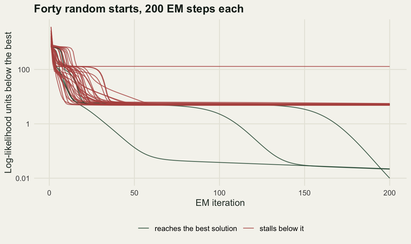
The picture shows something the summary table cannot. The runs drop fast and then stop on a shared plateau some way short of the best, but they do not all arrive at once: at iteration fifteen they are still spread over more than an order of magnitude, several of them holding a much higher ledge, and the slowest of the stalled runs is still edging down almost to the end of the plot. Some of the runs that eventually escape sit on that plateau first, and how long they sit there, and how late the last of them breaks away, change from one dataset of this design to the next. A convergence rule that stops when the change per step gets small can call such a run finished on the plateau, well before it has found anything. This is the practical hazard of EM on mixtures: a flat stretch looks exactly like convergence.
Taking the start that got furthest and running it properly gives the fit the rest of the post uses.
sb <- st_s[[which.max(ll_s)]]
fit <- em_fit(len, sb$mu, sb$sg, rep(1 / n_age, n_age),
              tol = 1e-6, maxit = 3000)

print(round(c(iterations = fit$iter, converged = fit$converged,
              loglik = fit$loglik), 3))
iterations converged loglik
413.000 1.000 -6427.314 print(round(rbind(mu_hat = fit$mu, mu_true = mu_true,
sd_hat = fit$sg, sd_true = sd_true,
p_hat = fit$w, p_true = p_true), 3)) [,1] [,2] [,3] [,4]
mu_hat 19.541 29.917 37.761 43.787
mu_true 19.516 29.891 37.733 43.659
sd_hat 1.372 2.013 2.583 2.777
sd_true 1.366 2.092 2.641 3.056
p_hat 0.396 0.280 0.196 0.128
p_true 0.392 0.276 0.195 0.137d_b <- diff(fit$trace)
print(c(min_increment = format(min(d_b), digits = 4),
any_decrease = as.character(any(d_b < 0))))min_increment any_decrease
"9.972e-07" "FALSE" fit_t <- em_fit(len, mu_true, sd_true, p_true, tol = 1e-6, maxit = 3000)
print(round(c(truth_start_iter = fit_t$iter,
truth_start_loglik = fit_t$loglik), 3)) truth_start_iter truth_start_loglik
549.000 -6427.314 print(round(c(max_mu_error = max(abs(fit$mu - mu_true)),
p4_shortfall = p_true[4] - fit$w[4]), 3))max_mu_error p4_shortfall
0.128 0.009 print(round(c(p4_shortfall_fish = n_fish * (p_true[4] - fit$w[4])), 1))p4_shortfall_fish
17.8 413 iterations to meet the same tolerance on the change in log-likelihood, with the smallest increment along the way 9.972e-07 and no decrease anywhere. The estimated mean lengths are 19.541, 29.917, 37.761 and 43.787 cm against a truth of 19.516, 29.891, 37.733 and 43.659. The largest error is 0.128 cm, on the fourth component. Proportions come back as 0.396, 0.28, 0.196 and 0.128 against 0.392, 0.276, 0.195 and 0.137, so the oldest class is underestimated by 0.009 in proportion, about 17.8 fish.
Starting EM at the true parameter values, which is a luxury nobody has with real data, reaches the same log-likelihood of -6427.314 after 549 iterations. Two very different starting points arriving at the same place is decent evidence that this is the best interior fit rather than another plateau.
The standard deviations are the weak part of the fit. The truth for the third and fourth components is 2.641 and 3.056 cm; the estimates are 2.583 and 2.777. Both are too narrow, and they are too narrow together, which is what happens when two heavily overlapping components divide up a shoulder: the fit can move mass between them and pull both in without losing much likelihood.
grid_len <- seq(min(len) - 1, max(len) + 1, length.out = 500)
comp_dat <- do.call(rbind, lapply(seq_len(n_age), function(k)
  data.frame(length_cm = grid_len,
             density = fit$w[k] * dnorm(grid_len, fit$mu[k], fit$sg[k]),
             component = paste("age", k))))
tot_dat <- data.frame(length_cm = grid_len,
                      density = rowSums(dens_mat(grid_len, fit$mu,
                                                 fit$sg, fit$w)),
                      series = "mixture total")

ggplot() +
  geom_histogram(data = data.frame(length_cm = len),
                 aes(x = length_cm, y = after_stat(density)),
                 binwidth = 0.5, fill = te_pal$line, colour = NA) +
  geom_line(data = comp_dat, aes(length_cm, density, colour = component),
            linewidth = 0.8) +
  geom_line(data = tot_dat, aes(length_cm, density, linetype = series),
            colour = te_pal$ink, linewidth = 1) +
  scale_colour_manual(values = comp_col, name = NULL) +
  scale_linetype_manual(values = c("mixture total" = "22"), name = NULL) +
  labs(x = "Length (cm)", y = "Density",
       title = "Fitted four component mixture") +
  theme_te()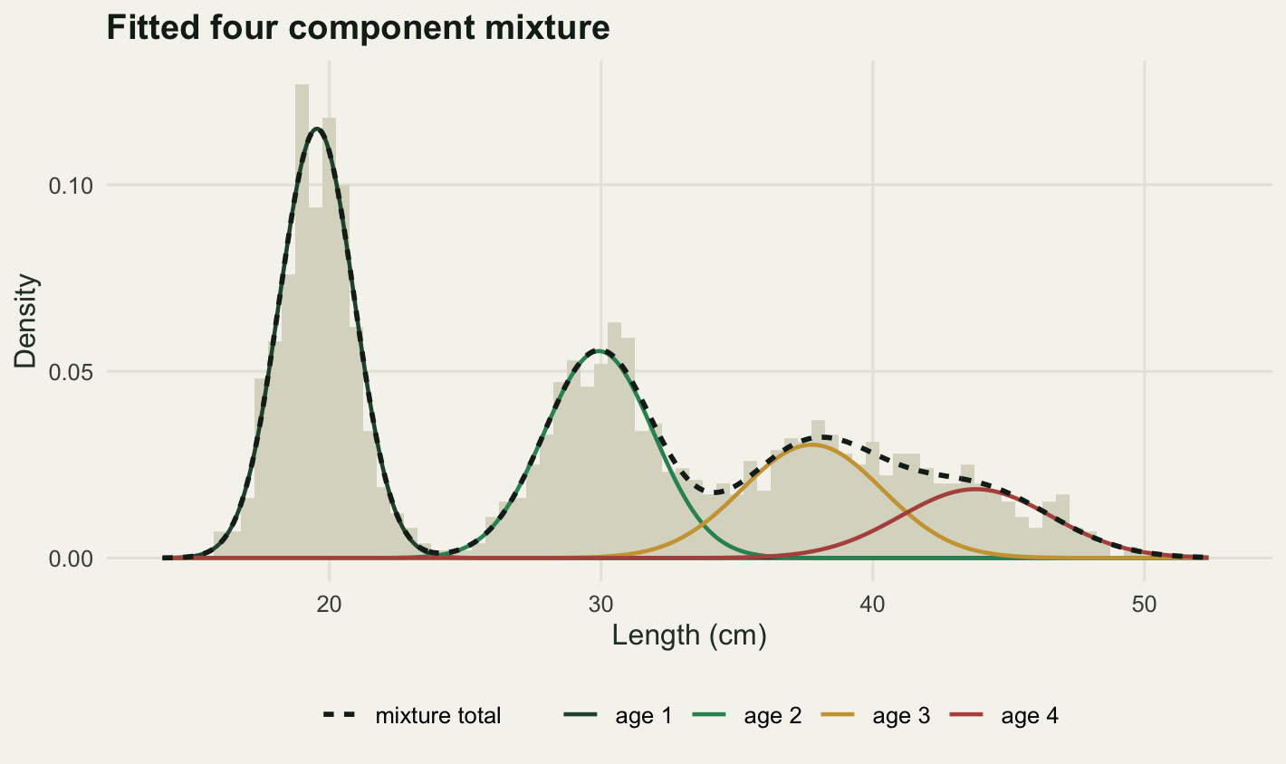
The picture makes the difficulty obvious in a way the numbers do not. The first two components are drawn under obvious peaks and the third under a much fainter one: the histogram dips in the middle of the shoulder and then rises into a low bump, and the fitted total keeps both. The fourth is drawn under no feature at all, a declining tail with nothing in it, so its position is decided almost entirely by the assumption that each age class is normal rather than by anything in the data. If that assumption is wrong the tail can be divided up in many other ways, and the histogram will not object.
The likelihood has no maximum
There is a worse problem than local maxima, and it is easy to miss because a fitting routine that returns a sensible answer never mentions it. For a mixture of normals with unrestricted, component-specific variances, the likelihood is unbounded. Put one component’s mean exactly on an observed value and let its standard deviation go to zero: that fish’s density contribution grows without limit while the other fish carry on being fitted by the remaining components.
The demonstration takes the fitted model, adds a fifth component with a weight of 0.002 centred on one particular fish, and evaluates the log-likelihood as the spike gets narrower.
spike_i <- which.min(abs(len - 33))
eps <- 0.002
sd_grid <- c(1, 0.1, 0.01, 1e-3, 1e-4, 1e-5, 1e-6)

ll_spike <- sapply(sd_grid, function(s)
  sum(log(rowSums(dens_mat(len,
                           c(fit$mu, len[spike_i]),
                           c(fit$sg, s),
                           c(fit$w * (1 - eps), eps))))))

print(data.frame(spike_sd = sd_grid, loglik = round(ll_spike, 2)))
spike_sd loglik
1 1e+00 -6427.42
2 1e-01 -6427.81
3 1e-02 -6429.33
4 1e-03 -6427.73
5 1e-04 -6425.46
6 1e-05 -6423.16
7 1e-06 -6420.85print(round(c(best_loglik = fit$loglik,
per_decade = mean(diff(ll_spike[4:7])),
log_10 = log(10), spike_fish_length = len[spike_i],
spike_weight = eps), 3)) best_loglik per_decade log_10 spike_fish_length
-6427.314 2.293 2.303 32.990
spike_weight
0.002 print(round(c(gain_over_best_fit = ll_spike[7] - fit$loglik), 2))gain_over_best_fit
6.46 At a spike width of 1 cm the addition costs a little: the log-likelihood is -6427.42 against -6427.314 for the fitted model, because the 0.002 of probability mass taken from the four real components is worth more where it was. The cost peaks at a width of 0.01 cm, where the log-likelihood is -6429.33. Below that the spike’s own fish starts to dominate and the log-likelihood turns around and climbs through -6425.46, -6423.16 and -6420.85 as the width falls by successive factors of ten, ending 6.46 units above the best interior fit.
It never stops. Each factor of ten narrower adds 2.293 to the log-likelihood over this stretch of the grid, which is the natural log of ten, 2.303, to within a hundredth. That is not a coincidence: the density at the centre of a normal is proportional to one over its standard deviation, and the log of that is minus the log of the width. The supremum of the likelihood is infinite and there is no maximum likelihood estimate to find. Kiefer and Wolfowitz described exactly this in 1956; Day set it out for the normal mixture case in 1969.
EM walks straight into it if you let it start there.
sp_mu <- c(fit$mu, len[spike_i])
sp_sd <- c(fit$sg, 1e-3)
sp_w <- c(fit$w * (1 - eps), eps)

dm_sp <- dens_mat(len, sp_mu, sp_sd, sp_w)
post_sp <- dm_sp / rowSums(dm_sp)
nk_sp <- colSums(post_sp)
mu_sp <- crossprod(post_sp, len)[, 1] / nk_sp
v_sp <- crossprod(post_sp, len^2)[, 1] / nk_sp - mu_sp^2

print(round(c(spike_membership = nk_sp[5], spike_new_mean = mu_sp[5],
              spike_new_variance = v_sp[5],
              fish_length = len[spike_i]), 6))
spike_membership spike_new_mean spike_new_variance fish_length
0.972269 32.989845 0.000000 32.989845 One M step from a spike one thousandth of a centimetre wide gives it a membership of 0.972269 fish, a new mean of 32.989845 cm, which is that one fish’s length to six decimal places, and a new variance of 0 to the same precision. The next E step divides by that standard deviation, which is now zero. The log-likelihood becomes infinite and every subsequent quantity is undefined. The algorithm has not failed: it has found the supremum, and the supremum is useless.
Two repairs are standard. The first is a floor on the standard deviation, which is what the sd_floor argument in em_fit does. The second is to force all components to share one variance, which makes the likelihood bounded because no single component can collapse without dragging the others with it.
spike_start <- list(
  mu = c(len[spike_i], as.numeric(quantile(len, c(0.3, 0.6, 0.9)))),
  sg = c(1e-3, rep(sd(len) / 2, 3)),
  w = c(eps, rep((1 - eps) / 3, 3)))

fit_fl <- em_fit(len, spike_start$mu, spike_start$sg, spike_start$w,
                 tol = 1e-6, maxit = 2000, sd_floor = 0.4)
print(round(c(floor = 0.4, iterations = fit_fl$iter,
              loglik = fit_fl$loglik), 3))
floor iterations loglik
0.400 69.000 -6433.652 print(signif(rbind(mu = fit_fl$mu, sd = fit_fl$sg, p = fit_fl$w), 4)) [,1] [,2] [,3] [,4]
mu 19.5400 29.7500 3.335e+01 39.4800
sd 1.3730 1.9100 4.000e-01 4.4960
p 0.3958 0.2525 3.965e-07 0.3517fit_eq <- em_fit(len, spike_start$mu, spike_start$sg, spike_start$w,
tol = 1e-6, maxit = 2000, equal_var = TRUE)
print(round(c(iterations = fit_eq$iter, loglik = fit_eq$loglik), 3))iterations loglik
62.000 -6519.676 print(round(rbind(mu = fit_eq$mu, sd = fit_eq$sg, p = fit_eq$w), 3)) [,1] [,2] [,3] [,4]
mu 19.575 30.095 38.009 44.324
sd 1.865 1.865 1.865 1.865
p 0.398 0.289 0.193 0.120set.seed(70518824)
ll_eq <- numeric(n_start); it_eq <- integer(n_start)
for (s in seq_len(n_start)) {
st <- list(mu = sample(len, n_age), sg = rep(sd(len) / 2, n_age))
f <- em_fit(len, st$mu, st$sg, rep(1 / n_age, n_age),
tol = 1e-6, maxit = 2000, equal_var = TRUE)
ll_eq[s] <- f$loglik; it_eq[s] <- f$iter
}
print(round(c(eq_best = max(ll_eq), eq_distinct = length(unique(round(ll_eq, 1))),
eq_within_1 = sum(ll_eq > max(ll_eq) - 1),
eq_median_iter = median(it_eq),
free_within_1 = sum(ll_s > max(ll_s) - 1),
min_sd_at_best_fit = min(fit$sg)), 3)) eq_best eq_distinct eq_within_1 eq_median_iter
-6519.676 3.000 17.000 44.500
free_within_1 min_sd_at_best_fit
3.000 1.372 print(round(c(floor_sd_comp3 = fit_fl$sg[3]), 3))floor_sd_comp3
0.4 print(round(c(floor_fish_comp3 = n_fish * fit_fl$w[3]), 6))floor_fish_comp3
0.000793 print(round(c(floor_loglik_cost = fit$loglik - fit_fl$loglik,
equal_var_loglik_cost = fit$loglik - max(ll_eq),
mu_error_free = mean(abs(fit$mu - mu_true)),
mu_error_equal_var = mean(abs(fit_eq$mu - mu_true))), 3)) floor_loglik_cost equal_var_loglik_cost mu_error_free
6.339 92.362 0.052
mu_error_equal_var
0.301 The floor of 0.4 cm does its job in the narrow sense: the run finishes in 69 iterations at a finite log-likelihood of -6433.652 instead of diverging. It does not give a usable fit. The third component sits on the floor at a standard deviation of 0.4 cm with a proportion of 3.965e-07, which is 0.000793 of a fish: the spike survived as a dead component pinned at its minimum width, and the remaining three components had to cover the data on their own, ending 6.339 units below the best fit. A variance floor stops the algorithm running off the edge. It does nothing about local maxima, and it leaves rubbish in the parameter vector that you have to notice yourself.
The equal-variance constraint behaves better and is more interesting. From the same poisoned start it converges in 62 iterations to a common standard deviation of 1.865 cm and means of 19.575, 30.095, 38.009 and 44.324 cm. Run from the same forty random starts as before, and given two thousand steps each rather than the two hundred the earlier run was capped at, it converges to 3 distinct log-likelihood values, and 17 of the forty reach its best answer against 3 for the unrestricted model, in a median of 44.5 iterations rather than hundreds.
That is a genuine trade and it does not go the way the fit statistics suggest. The equal-variance model is 92.362 log-likelihood units worse and it is plainly false here, since the simulated standard deviations really do run from 1.366 to 3.056 cm. Its mean lengths are further from the truth on average, 0.301 cm against 0.052 cm for the unrestricted fit. What it buys is an answer you can actually reproduce. On a survey you cannot check against a simulated truth, that reproducibility is worth more than it looks.
The floor, incidentally, never binds at the good solution. The smallest fitted standard deviation there is 1.372 cm, well clear of 0.4, so adding the floor to the multi-start recipe costs nothing at the answer you want and removes the one place the algorithm can fall off. Floor plus many starts is the working combination.
Soft classification is the output
What EM returns for each fish is not an age. It is a row of four probabilities. The matrix of those rows is the post element of the fit, and looking at it is the quickest way to understand what a mixture model can and cannot tell you about an individual.
post <- fit$post
max_post <- apply(post, 1, max)
hard <- apply(post, 1, which.max)

print(round(c(median_max_post = median(max_post),
              frac_below_0.9 = mean(max_post < 0.9),
              frac_below_0.8 = mean(max_post < 0.8),
              frac_below_0.6 = mean(max_post < 0.6),
              n_below_0.8 = sum(max_post < 0.8),
              accuracy = mean(hard == true_age)), 4))
median_max_post frac_below_0.9 frac_below_0.8 frac_below_0.6 n_below_0.8
0.9972 0.1895 0.1180 0.0380 236.0000
accuracy
0.9320 print(round(apply(post, 2, max), 4))[1] 1.0000 0.9998 0.9693 0.9999print(round(tapply(hard == true_age, true_age, mean), 3)) 1 2 3 4
1.000 0.964 0.849 0.785 print(round(c(pct_below_0.8 = 100 * mean(max_post < 0.8),
pct_below_0.6 = 100 * mean(max_post < 0.6)), 2))pct_below_0.8 pct_below_0.6
11.8 3.8 print(round(c(pct_max_for_age3 = 100 * max(post[, 3])), 1))pct_max_for_age3
96.9 The median fish is assigned with probability 0.9972, which sounds like the problem is solved. It is the tail that matters. 11.8 per cent of the fish, that is 236 of them, have no class with a posterior above 0.8, and 3.8 per cent have none above 0.6. For those fish the model is close to saying it does not know.
The largest posterior probability that any fish anywhere on the length axis achieves for each component is the sharpest single measurement in this post. For the third component that maximum is 0.9693. There is no length at all at which a fish can be called a three-year-old with more than 96.9 per cent confidence, because the third component is overlapped on the left by the second and on the right by the fourth and never gets a stretch of the axis to itself. Assignment accuracy against the known truth falls from 1 for age 1 to 0.785 for age 4.
post_grid <- dens_mat(grid_len, fit$mu, fit$sg, fit$w)
post_grid <- post_grid / rowSums(post_grid)
post_dat <- do.call(rbind, lapply(seq_len(n_age), function(k)
  data.frame(length_cm = grid_len, prob = post_grid[, k],
             component = paste("age", k))))

ggplot(post_dat, aes(length_cm, prob, colour = component)) +
  geom_hline(yintercept = 0.8, colour = te_pal$ink,
             linetype = "22", linewidth = 0.4) +
  geom_line(linewidth = 0.9) +
  geom_rug(data = data.frame(length_cm = len[max_post < 0.8]),
           aes(x = length_cm), sides = "b", colour = te_pal$ink,
           alpha = 0.25, inherit.aes = FALSE) +
  scale_colour_manual(values = comp_col, name = NULL) +
  labs(x = "Length (cm)", y = "Posterior membership probability",
       title = "Which age class does a fish of this length belong to") +
  theme_te()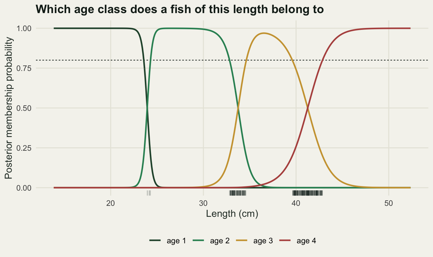
The three bands of rug marks are the boundaries between age classes, and their widths are the honest measure of how much a length tells you. The gap between the one-year-olds and the two-year-olds is a knife edge: only a few fish land in it. The gap between ages three and four is a wide grey zone several centimetres across, and the age 3 curve is the only one that never reaches the top of the panel.
Now for the thing that actually gets done with a fit like this. Catch at age is a vector of how many fish in the sample belong to each age class, and it feeds directly into a stock assessment. There are two ways to build it: assign each fish to its most probable class and count, or add up the posterior probabilities column by column and never assign anybody.
caa_true <- tabulate(true_age, n_age)
caa_hard <- tabulate(hard, n_age)
caa_soft <- colSums(post)

print(round(rbind(truth = caa_true, hard = caa_hard, soft = caa_soft,
                  n_times_p_hat = n_fish * fit$w), 2))
[,1] [,2] [,3] [,4]
truth 791.00 560.00 370.00 279.00
hard 791.00 568.00 394.00 247.00
soft 791.46 559.25 392.74 256.55
n_times_p_hat 791.46 559.25 392.73 256.56print(round(rbind(error_hard = caa_hard - caa_true,
error_soft = caa_soft - caa_true), 2)) [,1] [,2] [,3] [,4]
error_hard 0.00 8.00 24.00 -32.00
error_soft 0.46 -0.75 22.74 -22.45print(round(c(mae_hard = mean(abs(caa_hard - caa_true)),
mae_soft = mean(abs(caa_soft - caa_true)),
rmse_hard = sqrt(mean((caa_hard - caa_true)^2)),
rmse_soft = sqrt(mean((caa_soft - caa_true)^2)),
worst_hard = max(abs(caa_hard - caa_true)),
worst_soft = max(abs(caa_soft - caa_true)),
soft_minus_np = max(abs(caa_soft - n_fish * fit$w))), 3)) mae_hard mae_soft rmse_hard rmse_soft worst_hard
16.000 11.600 20.396 15.985 32.000
worst_soft soft_minus_np
22.742 0.008 print(round(c(worst_soft_1dp = max(abs(caa_soft - caa_true)),
age4_shortfall_hard = caa_true[4] - caa_hard[4],
age4_shortfall_soft = caa_true[4] - caa_soft[4],
mae_gain_fish = mean(abs(caa_hard - caa_true)) -
mean(abs(caa_soft - caa_true))), 1)) worst_soft_1dp age4_shortfall_hard age4_shortfall_soft mae_gain_fish
22.7 32.0 22.5 4.4 print(round(c(mae_reduction_pct = 100 * (1 - mean(abs(caa_soft - caa_true)) /
mean(abs(caa_hard - caa_true))),
best_over_quantile_fit = fit$loglik - fit_q$loglik), 2)) mae_reduction_pct best_over_quantile_fit
27.50 4.83 The two routes do not give the same answer. Mean absolute error across the four age classes is 11.6 fish for the soft version and 16 for the hard one, a gap of 27.5 per cent of the hard figure in favour of the soft route, and the worst single age class is out by 22.7 fish under the soft route compared with 32 under the hard one. Neither the size nor the sign of that gap belongs to the method. It is one draw of a sampling error, and another survey generated the same way can put the hard table ahead. Under hard assignment age 4 ends up short by 32 fish, and those fish turn up in the younger classes, because in the overlap zone every fish is handed whole to whichever component wins the argmax instead of being split between them.
The fourth row of the first table explains why the soft version is the better estimator. At an EM fixed point the M step sets each \(\pi_k\) to the mean of column \(k\) of the posterior matrix, so the summed posteriors and \(n\hat{\pi}\) are the same vector by construction: the largest discrepancy here is 0.008 fish, which is what stopping at a finite convergence tolerance leaves behind. The soft catch at age is the maximum likelihood estimate of the age composition. The hard one is a different estimator that nobody derived, and it is biased in a direction set by the shapes of the components.
What that argument does not do is rescue either estimate. At age 4 the truth minus the estimate comes to 32 fish for hard assignment and 22.5 for soft, and the soft figure is what the fitted \(\pi_4\) gets wrong and nothing else, since the soft count is \(n\hat{\pi}_4\) by construction. Soft assignment removes the error from rounding the classifications. It cannot remove an error that is already in the parameters.
err_dat <- data.frame(
  age = rep(factor(seq_len(n_age)), 2),
  error = c(caa_hard - caa_true, caa_soft - caa_true),
  method = rep(c("hard assignment", "summed posteriors"), each = n_age))

ggplot(err_dat, aes(age, error, fill = method)) +
  geom_hline(yintercept = 0, colour = te_pal$ink, linewidth = 0.4) +
  geom_col(position = position_dodge(width = 0.75), width = 0.65) +
  scale_fill_manual(values = c(te_pal$clay, te_pal$green), name = NULL) +
  labs(x = "Age class", y = "Estimated minus true number of fish",
       title = "Catch at age, hard against soft") +
  theme_te()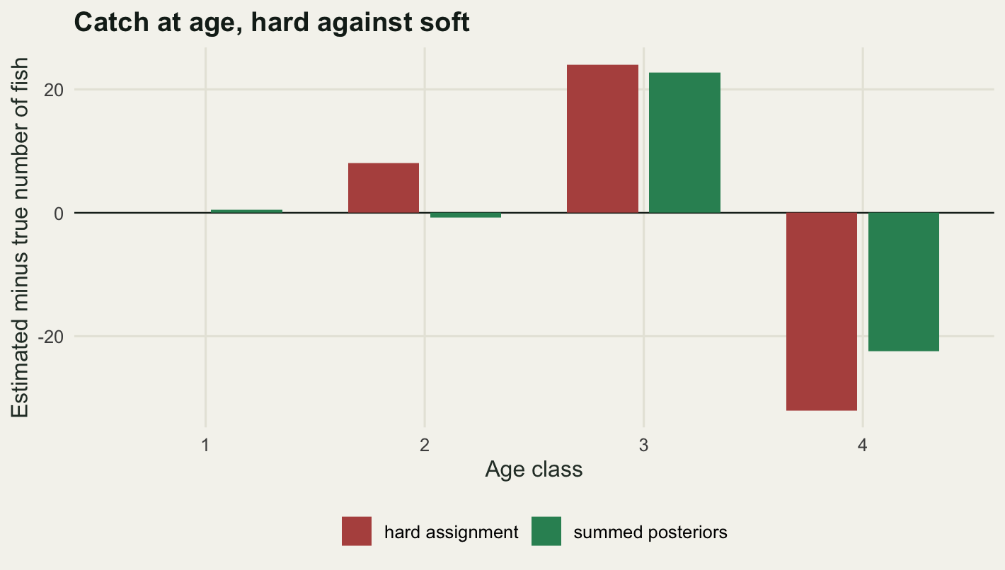
Standard errors, two ways
EM gives no standard errors. The quantities it computes along the way belong to the complete-data likelihood, the one that pretends the labels are known, and the curvature of that surface is not the curvature of the surface that was actually maximised. Using it would give intervals that are too narrow, sometimes very much too narrow.
The direct fix is to write down the observed-data log-likelihood as a function of the parameter vector and differentiate it numerically. optimHess does that in base R with central differences: no optimisation, just the Hessian at a point you supply. The parameter vector below is four means, four standard deviations and three of the four proportions, eleven free parameters in all.
neg_ll <- function(th) {
  mu <- th[1:n_age]
  sg <- th[n_age + 1:n_age]
  pr <- c(th[2 * n_age + seq_len(n_age - 1)], 0)
  pr[n_age] <- 1 - sum(pr)
  if (any(sg <= 0) || any(pr <= 0)) return(1e10)
  -sum(log(rowSums(dens_mat(len, mu, sg, pr))))
}

th_hat <- c(fit$mu, fit$sg, fit$w[-n_age])
hess <- optimHess(th_hat, neg_ll,
                  control = list(ndeps = rep(1e-4, length(th_hat))))
se_hess <- sqrt(diag(solve(hess)))
print(round(c(n_par = length(th_hat), check = neg_ll(th_hat) + fit$loglik), 6))
n_par check
1.1e+01 -1.0e-06 The parametric bootstrap answers the same question by brute force. Simulate a fresh sample of the same size from the fitted model, refit it, and repeat; the standard deviation of the replicate estimates is the standard error. Fifty replicates is a small number, chosen to keep this post’s runtime down, and it means each standard error below is itself uncertain by roughly ten per cent. Each replicate is started at the fitted values, which is the usual shortcut and which assumes the replicate optimum is near the original.
set.seed(50311907)
n_boot <- 50
boot <- matrix(NA_real_, n_boot, length(th_hat))

for (b in seq_len(n_boot)) {
  a <- sample(n_age, n_fish, replace = TRUE, prob = fit$w)
  x_b <- rnorm(n_fish, fit$mu[a], fit$sg[a])
  f_b <- em_fit(x_b, fit$mu, fit$sg, fit$w, tol = 1e-5, maxit = 800)
  boot[b, ] <- c(f_b$mu, f_b$sg, f_b$w[-n_age])
}
se_boot <- apply(boot, 2, sd)

print(data.frame(
  parameter = c(paste0("mu", seq_len(n_age)), paste0("sd", seq_len(n_age)),
                paste0("p", seq_len(n_age - 1))),
  estimate = round(th_hat, 3),
  se_hessian = round(se_hess, 3),
  se_boot = round(se_boot, 3),
  ratio = round(se_hess / se_boot, 2)))
parameter estimate se_hessian se_boot ratio
1 mu1 19.541 0.049 0.047 1.05
2 mu2 29.917 0.158 0.164 0.97
3 mu3 37.761 0.860 0.541 1.59
4 mu4 43.787 1.589 1.144 1.39
5 sd1 1.372 0.036 0.033 1.11
6 sd2 2.013 0.115 0.112 1.02
7 sd3 2.583 0.769 0.667 1.15
8 sd4 2.777 0.594 0.485 1.23
9 p1 0.396 0.011 0.012 0.93
10 p2 0.280 0.016 0.017 0.95
11 p3 0.196 0.079 0.060 1.33print(round(c(n_boot = n_boot, max_ratio = max(se_hess / se_boot),
min_ratio = min(se_hess / se_boot),
boot_median_mu4 = median(boot[, 4]),
estimate_mu4 = th_hat[4]), 3)) n_boot max_ratio min_ratio boot_median_mu4 estimate_mu4
50.000 1.589 0.926 44.082 43.787 For the two well-separated components the two methods agree to within a few per cent. The mean of the first component has a Hessian standard error of 0.049 cm and a bootstrap standard error of 0.047; for the second the pair is 0.158 and 0.164. The first two proportions agree just as well. If the post stopped there the conclusion would be that either method is fine.
They disagree badly on exactly the parameters that matter for the hard part of the problem, and they disagree in the direction opposite to the usual warning. The received advice about asymptotic standard errors is that they are optimistic. Here the numerical Hessian is the pessimistic one: 0.86 cm against 0.541 for the third mean, a ratio of 1.59, and 1.589 against 1.144 for the fourth, a ratio of 1.39. The third proportion goes the same way, 0.079 against 0.06. Across all eleven parameters the ratio runs from 0.93 to 1.59.
Neither number is wrong; they are answers to different questions. The Hessian measures the curvature of the log-likelihood at one point, and along the ridge that trades the third component against the fourth that surface is almost flat, so the quadratic approximation opens out into a very wide bell. The bootstrap measures how far the estimates actually move when new data arrive from the fitted model, and the likelihood falls away faster than the quadratic once you leave the immediate neighbourhood of the peak, so the replicates do not travel as far as the curvature predicts. The bootstrap distribution is also not centred on the estimate: its median for the fourth mean is 44.082 cm against an estimate of 43.787, so a symmetric interval built from either standard error is misplaced as well as mis-scaled.
The practical reading is that for the poorly separated components you should not report a standard error at all. A percentile interval from a larger bootstrap, or a profile likelihood, will describe an asymmetric and very wide uncertainty honestly, whereas a single standard error multiplied by the usual normal quantile will not.
What to take away
The mechanics are genuinely simple. An E step that is Bayes’ theorem, an M step that is three weighted averages, a loop, and a convergence check on a log-likelihood guaranteed never to decrease. Everything hard about mixture models is elsewhere: they have many local maxima and EM finds whichever one is nearest, they have no maximum likelihood estimate at all when variances are free, and long flat stretches in the log-likelihood look like convergence from the inside. The working recipe is many random starts, a floor on the variances, and enough iterations that you are sure the plateau is the top rather than a ledge.
The output is soft, and it should be kept soft. Individual fish in the overlap zones carry real information about the age composition even when nobody can say what age they are, and the summed posterior probabilities are the maximum likelihood estimate of that composition while a table of hard assignments is not. That is the whole of the argument, and it says nothing about the size of the error gap: the hard table’s mean absolute error minus the soft one’s is 4.4 fish per age class, and on a single survey that difference can fall on either side of zero. Which route the arithmetic happens to favour on one sample is a different question from which one estimates the composition, and the moment a fish is given a single age the information is gone for good.
The honest limit is this: a mixture of normals is a description of the shape of a distribution and nothing more, and it becomes an age key only if the biological story behind it is true. This post generated the data from four Gaussian age classes and then recovered four Gaussian age classes, which proves the arithmetic works and proves nothing about any real fish. The same shoulder on the right of a real histogram can be produced by three overlapping cohorts, by five, or by a single skewed distribution of lengths with no cohort structure in it whatsoever, and the fitted log-likelihood will not settle the argument. It compares fits that carry the same number of components, and on that comparison the four-component fit this post kept came out 4.83 units clear of the one that put two components inside the same peak. Across different numbers of components it climbs whatever produced the data, so it cannot say how many cohorts there are to find. Choosing the number of components, and telling a mixture apart from a skewed distribution, are separate problems that need separate tools; they are the subjects of the next two posts in this series.
References
Dempster AP, Laird NM, Rubin DB 1977 Journal of the Royal Statistical Society Series B 39(1):1-22 (10.1111/j.2517-6161.1977.tb01600.x)
Macdonald PDM, Pitcher TJ 1979 Journal of the Fisheries Research Board of Canada 36(8):987-1001 (10.1139/f79-137)
Day NE 1969 Biometrika 56(3):463-474 (10.1093/biomet/56.3.463)
Hasselblad V 1966 Technometrics 8(3):431-444 (10.1080/00401706.1966.10490375)
Kiefer J, Wolfowitz J 1956 The Annals of Mathematical Statistics 27(4):887-906 (10.1214/aoms/1177728066)
McLachlan GJ, Peel D 2000 Finite Mixture Models (ISBN 978-0-471-00626-8)