library(ggplot2)
library(patchwork)

te_paper  <- "#f5f4ee"
te_ink    <- "#16241d"
te_body   <- "#2c3a31"
te_forest <- "#275139"
te_rust   <- "#b5534e"
te_gold   <- "#c9b458"
te_line   <- "#dad9ca"

theme_datasheet <- function() {
  theme_minimal(base_size = 12) +
    theme(plot.background  = element_rect(fill = te_paper, colour = NA),
          panel.background = element_rect(fill = te_paper, colour = NA),
          panel.grid.major = element_line(colour = te_line, linewidth = 0.3),
          panel.grid.minor = element_blank(),
          text             = element_text(colour = te_body),
          plot.title       = element_text(colour = te_ink, face = "bold"),
          plot.subtitle    = element_text(colour = te_body),
          axis.text        = element_text(colour = te_body))
}Borrowed age-length keys and strong year classes
R
fisheries
age structure
EM
simulation
ecology tutorial
An age-length key borrowed from another year halves a strong year class. In R: the exact forward bias, the inverse EM key, and where a growth curve fixes it.
A demersal trawl survey measures every fish it catches, a couple of thousand lengths a year, but otoliths are expensive to read and the ageing laboratory is behind. The age composition for this year still has to go into the assessment. A common stopgap is to apply a key from an earlier year (or pooled years), the table of how many fish of each length turned out to be of each age, to this year’s length frequency. The growth of the species has not changed, so the key looks like a property of the fish.
It is not. A forward key gives the probability of an age given a length, and that probability depends on how many fish of each age were in the population the key was built from. Westrheim and Ricker showed in 1978 that a key carried to a population with a different age structure pulls the estimated composition back toward the population it came from. The fix that followed was to turn the key around: estimate the probability of a length given an age from the aged fish, which does not depend on the age structure, and recover the new year’s age proportions from its length frequency by iteration. Kimura and Chikuni gave that iterative key in 1987, and Hoenig and Heisey in the same year gave a log-linear EM formulation that also re-estimates the length-at-age table from the unaged fish. None of this is new, and this post is a demonstration of those papers rather than a finding of its own. What it measures is the price of the inverse key, and where its remaining bias comes from.
The neighbours on this site stop short of the key. Fitting a mixture of normals in R takes a length sample with the ages taken out altogether and separates the age classes with EM and no aged fish at all; here some fish are aged, and the question is what happens when their ages come from the wrong year. Stock-recruitment and reference points fits catch curves to an age composition that comes either from a noisy grid or from ageing a finite sample of fish, which is sampling noise with no key transfer. Fishing, age truncation and spawning variability works with ages known exactly. The last section below comes back to the catch curve, because total mortality is what most age compositions are for.
Two years of the same stock
The design constants come first, all in one chunk.
ages     <- 1:8
n_age    <- length(ages)
l_inf    <- 60        # asymptotic length, cm
k_growth <- 0.3       # von Bertalanffy growth coefficient
t_zero   <- -0.3      # age at length zero
cv_len   <- 0.12      # coefficient of variation of length at age
z_mort   <- 0.35      # total mortality behind year A's age structure
mean_len <- l_inf * (1 - exp(-k_growth * (ages - t_zero)))
sd_len   <- cv_len * mean_len

prop_a <- exp(-z_mort * ages)
prop_a <- prop_a / sum(prop_a)

bin_width <- 2
brks      <- seq(0, 80, by = bin_width)
n_bin     <- length(brks) - 1

bin_probs <- function(mu, s) {
  p_mat <- sapply(seq_along(mu), function(a) diff(pnorm(brks, mu[a], s[a])))
  sweep(p_mat, 2, colSums(p_mat), "/")
}
len_given_age <- bin_probs(mean_len, sd_len)   # bins by ages, columns sum to one

year_b_props <- function(strong_age, strength) {
  p_vec <- prop_a
  p_vec[strong_age] <- p_vec[strong_age] * strength
  p_vec / sum(p_vec)
}

draw_fish <- function(n, p_age) {
  a_vec <- sample.int(n_age, n, replace = TRUE, prob = p_age)
  l_vec <- rnorm(n, mean_len[a_vec], sd_len[a_vec])
  l_vec <- pmin(pmax(l_vec, 0.01), 79.99)
  list(age = a_vec, len = l_vec, bin = findInterval(l_vec, brks))
}

n_meas     <- 2000
strong_use <- 4
mult_use   <- 4
prop_b     <- year_b_props(strong_use, mult_use)
share_true <- prop_b[strong_use]
overlap_4  <- sum(pmin(len_given_age[, 3], len_given_age[, 4]))
overlap_6  <- sum(pmin(len_given_age[, 5], len_given_age[, 6]))
gap_46     <- mean_len[5] - mean_len[4]
gap_67     <- mean_len[7] - mean_len[6]

aged_use    <- 400                # fish aged in the headline case
aged_grid   <- c(200, 400, 1000)
n_rep_main  <- 300                # surveys per aged sample size
n_rep_grid  <- 100                # surveys per cell of the age by strength grid
expected_a4 <- aged_use * prop_a[strong_use]
gap_tol     <- 1e-5               # accepted distance from the likelihood maximum
n_bins_4    <- 4 * sd_len[strong_use] / bin_width
The simulated stock has eight age classes and one growth curve, a von Bertalanffy curve with asymptotic length 60 cm, growth coefficient 0.3 and a coefficient of variation of length at age of 0.12. Lengths are binned to 2 cm. In year A recruitment has been even, so the age structure is a geometric decline with total mortality 0.35. Year A supplies the aged fish. Year B has the same growth and the same mortality, but one year class is stronger than the others: in the headline case the fish of age 4 are 4 times as numerous as even recruitment would give. That class makes up 0.331 of year B, against 0.110 in year A.
All of these values, the 2000 fish measured in year B, and the grids further down were fixed before any estimator was run. One property of the growth curve matters later. Successive mean lengths close up with age: the age 4 and age 5 means are 4.3 cm apart and the age 6 and age 7 means only 2.3 cm, while the spread within an age grows. The length distributions of ages 3 and 4 share 0.56 of their probability; those of ages 5 and 6 share 0.79.
The borrowed key is a matrix product
With the true growth curve, the forward key of year A needs no simulation. Multiply the length-given-age table by year A’s age proportions, divide each length row by its total, and the rows are the probabilities of age given length. Year B’s expected length frequency is the same length-given-age table times year B’s proportions, and the key applied to that frequency is one more matrix product.
forward_exact <- function(p_from, p_to) {
  joint_from <- sweep(len_given_age, 2, p_from, "*")
  key_from   <- joint_from / pmax(rowSums(joint_from), 1e-300)   # P(age | length)
  len_to     <- len_given_age %*% p_to                            # length frequency
  as.vector(t(key_from) %*% len_to)
}
fwd_exact     <- forward_exact(prop_a, prop_b)
fwd_ratio     <- fwd_exact[strong_use] / share_true
same_exact    <- forward_exact(prop_b, prop_b)
same_gap      <- max(abs(same_exact - prop_b))
fwd_other_gap <- fwd_exact[-strong_use] - prop_b[-strong_use]

mult_grid  <- seq(1, 10, by = 0.25)
exact_grid <- do.call(rbind, lapply(c(2, 4, 6), function(sa) {
  data.frame(strong_age = sa, strength = mult_grid,
             ratio = vapply(mult_grid, function(m) {
               pb <- year_b_props(sa, m)
               forward_exact(prop_a, pb)[sa] / pb[sa]
             }, 0))
}))
ratio_at <- function(sa, m) exact_grid$ratio[exact_grid$strong_age == sa & exact_grid$strength == m]
The borrowed key gives age 4 an expected share of 0.154 against the true 0.331, a ratio of 0.467. The strong class keeps less than half of its share, and the fish taken from it go to ages 3 and 5 above all: their estimated shares are too high by 0.071 and 0.045. The same calculation with year B’s own key returns year B exactly, to within 2.78e-17. Nothing is wrong with the key as a description of year A; it is simply the wrong prior.
This is an infinite-sample result with the true growth curve, so it is also what any smoothed forward key built from year A converges to, whether the smoothing is a growth model or a multinomial regression of age on length. Smoothing reduces the noise of a forward key but cannot remove this bias, because the bias sits in the age proportions of the year the key came from. Gerritsen and colleagues model keys with a multinomial logistic regression, which fills empty length classes and lets keys be compared; their regional haddock keys differed through both length at age and relative abundance. The model is a better way to build or compare a key, not a way to transfer one.
The bias grows with the strength of the class and with its age. For a class twice the normal strength the ratio is 0.860 at age 2, 0.645 at age 4 and 0.602 at age 6; at eight times the normal strength it is 0.755, 0.378 and 0.303. Young fish overlap less in length, so the prior matters less, but even at age 2 an eight-fold class loses 24 per cent of its share; older fish overlap more and the prior decides.
len_mid <- brks[-1] - bin_width / 2
dens_df <- rbind(
  data.frame(len = len_mid, dens = as.vector(len_given_age %*% prop_a), year = "year A: even recruitment"),
  data.frame(len = len_mid, dens = as.vector(len_given_age %*% prop_b), year = "year B: age 4 four times stronger"))
p_age4   <- function(p_vec) { j <- sweep(len_given_age, 2, p_vec, "*"); j[, strong_use] / pmax(rowSums(j), 1e-300) }
key_long <- data.frame(len = len_mid, p = c(p_age4(prop_a), p_age4(prop_b)), year = rep(unique(dens_df$year), each = n_bin))
key_long <- key_long[key_long$len > 20 & key_long$len < 65, ]

p_len <- ggplot(dens_df, aes(len, dens / bin_width, colour = year)) +
  geom_line(linewidth = 0.9) +
  scale_colour_manual(values = c(te_forest, te_rust), name = NULL) +
  labs(x = "length (cm)", y = "density", title = "Length frequencies",
       subtitle = "expected, from the true growth curve") +
  theme_datasheet()
p_key <- ggplot(key_long, aes(len, p, colour = year)) +
  geom_line(linewidth = 0.9) +
  scale_colour_manual(values = c(te_forest, te_rust), name = NULL) +
  scale_y_continuous(limits = c(0, 1)) +
  labs(x = "length (cm)", y = "P(age 4 | length)", title = "The key for age 4",
       subtitle = "same growth, different age structure") +
  theme_datasheet()
p_len + p_key + plot_layout(guides = "collect") +
  plot_annotation(theme = theme_datasheet()) &
  theme(legend.position = "bottom", legend.direction = "horizontal")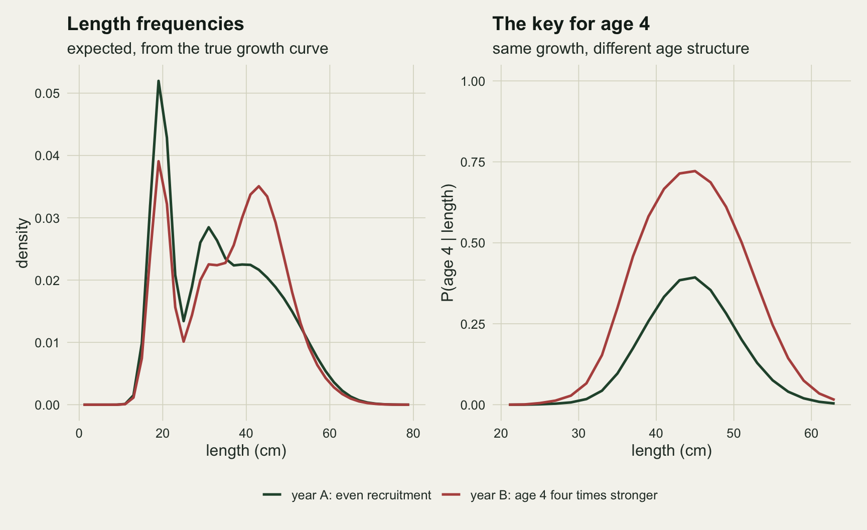
Simulated surveys: forward, same-year and inverse keys
The simulation draws, for each survey, 400 aged fish from year A, 2000 measured fish from year B, and a separate set of the same number of aged fish from year B for the same-year key. Five estimators are applied to the same year B lengths. The borrowed forward key and the same-year forward key are the usual count ratios. The inverse key uses year A’s aged fish only for the length distribution within each age, either as the raw proportions in each length bin (the empirical inverse key of Kimura and Chikuni) or as a fitted growth curve: a von Bertalanffy mean with a constant coefficient of variation, fitted by maximum likelihood to the individual lengths and ages, and converted to bin probabilities (the smoothed inverse key). A fifth arm uses the true length distributions as a control that no survey could have. Every inverse key is the maximum of the same likelihood, the one Kimura and Chikuni climb with EM. EM crawls when components overlap and a proportion belongs at zero, so the maximum is found here with Newton steps on a log barrier, and each fit is accepted only when a bound on its distance from the maximum (the largest gradient component minus the number of fish in length bins the key covers, in log-likelihood units) is below 0.00001. There are 300 surveys per aged sample size, and the aged sample size is 200, 400 or 1000 fish.
fit_vb <- function(age, len) {
  nll <- function(th) {
    mu <- exp(th[1]) * (1 - exp(-exp(th[2]) * (age - th[3])))
    if (any(mu <= 0)) return(1e10)
    -sum(dnorm(len, mu, exp(th[4]) * mu, log = TRUE))
  }
  th_start <- c(log(max(len)), log(0.3), 0, log(0.1))
  f_nm  <- optim(th_start, nll, control = list(maxit = 3000))
  f_bf  <- optim(f_nm$par, nll, method = "BFGS")
  mu    <- exp(f_bf$par[1]) * (1 - exp(-exp(f_bf$par[2]) * (ages - f_bf$par[3])))
  list(mu = mu, cv = exp(f_bf$par[4]), code = f_bf$convergence)
}

# one EM step of the inverse key (Kimura and Chikuni) for all surveys at once,
# kept as a check; q has one row per survey
em_step <- function(q, p_mat, counts, rid) {
  num <- p_mat * q[rid, , drop = FALSE]
  used <- rowsum(counts * (rowSums(p_mat) > 0), rid)[, 1]
  rowsum(num * (counts / pmax(rowSums(num), 1e-300)), rid) / used
}

# maximum of sum(counts * log(p_mat %*% q)) over proportions q:
# Newton steps on a log barrier whose weight falls from 10 to 1e-9
mix_mle <- function(p_mat, counts, max_newton = 200) {
  keep <- counts > 0 & rowSums(p_mat) > 0
  pm <- p_mat[keep, , drop = FALSE]
  cn <- counts[keep]
  q <- rep(1 / n_age, n_age)
  steps <- 0
  obj <- function(qq, mu) sum(cn * log(as.vector(pm %*% qq))) + mu * sum(log(qq))
  for (mu in 10^(1:-9)) {
    repeat {
      m_vec <- as.vector(pm %*% q)
      grad  <- colSums(pm * (cn / m_vec)) + mu / q
      h_inv <- solve(crossprod(pm * (sqrt(cn) / m_vec)) + diag(mu / q^2, n_age))
      d_vec <- as.vector(h_inv %*% grad - rowSums(h_inv) * sum(h_inv %*% grad) / sum(h_inv))
      decr  <- sum(d_vec * grad)
      if (decr < 1e-13 || steps >= max_newton) break
      t_step <- 1
      while (any(q + t_step * d_vec <= 0)) t_step <- t_step / 2
      f_now <- obj(q, mu)
      while (obj(q + t_step * d_vec, mu) < f_now + 0.25 * t_step * decr && t_step > 1e-10)
        t_step <- t_step / 2
      q <- q + t_step * d_vec
      q <- q / sum(q)
      steps <- steps + 1
    }
  }
  gap <- max(colSums(pm * (cn / as.vector(pm %*% q)))) - sum(cn)
  list(q = q, gap = gap, capped = steps >= max_newton)
}

fit_inverse <- function(p_mat, counts, n_rep) {
  fits <- lapply(seq_len(n_rep), function(r) {
    rows <- (r - 1) * n_bin + seq_len(n_bin)
    mix_mle(p_mat[rows, , drop = FALSE], counts[rows])
  })
  list(q = t(sapply(fits, `[[`, "q")), gap = sapply(fits, `[[`, "gap"),
       capped = sapply(fits, `[[`, "capped"))
}

catch_curve_z <- function(counts) {
  fit <- glm.fit(cbind(1, ages), counts, family = quasipoisson())
  -fit$coefficients[2]
}

run_cell <- function(n_rep, n_aged, strong_age, strength, arms) {
  pb <- year_b_props(strong_age, strength)
  lf  <- matrix(0, n_rep, n_bin)
  est <- list()
  if ("forward" %in% arms) est$forward <- matrix(0, n_rep, n_age)
  if ("same" %in% arms) est$same <- matrix(0, n_rep, n_age)
  true_b <- matrix(0, n_rep, n_age)
  p_emp <- p_smooth <- matrix(0, n_rep * n_bin, n_age)
  gap_share <- numeric(n_rep)
  for (r in seq_len(n_rep)) {
    fish_a <- draw_fish(n_aged, prop_a)
    fish_b <- draw_fish(n_meas, pb)
    rows   <- (r - 1) * n_bin + seq_len(n_bin)
    lf[r, ]     <- tabulate(fish_b$bin, n_bin)
    true_b[r, ] <- tabulate(fish_b$age, n_age) / n_meas
    tab_a <- table(factor(fish_a$bin, 1:n_bin), factor(fish_a$age, ages))
    if ("forward" %in% arms) {
      e_vec <- colSums(lf[r, ] * (tab_a / pmax(rowSums(tab_a), 1)))
      est$forward[r, ] <- e_vec / sum(e_vec)
    }
    if ("same" %in% arms) {
      fish_s <- draw_fish(n_aged, pb)
      tab_s  <- table(factor(fish_s$bin, 1:n_bin), factor(fish_s$age, ages))
      e_vec  <- colSums(lf[r, ] * (tab_s / pmax(rowSums(tab_s), 1)))
      est$same[r, ] <- e_vec / sum(e_vec)
    }
    p_emp[rows, ] <- sweep(tab_a, 2, pmax(colSums(tab_a), 1), "/")
    in_b <- fish_b$age == strong_age
    gap_share[r] <- mean(tab_a[cbind(fish_b$bin[in_b], strong_age)] == 0)
    vb <- fit_vb(fish_a$age, fish_a$len)
    p_smooth[rows, ] <- bin_probs(vb$mu, vb$cv * vb$mu)
  }
  counts <- as.vector(t(lf))
  fits <- list()
  if ("empirical" %in% arms) fits$empirical <- fit_inverse(p_emp, counts, n_rep)
  if ("smoothed" %in% arms)  fits$smoothed  <- fit_inverse(p_smooth, counts, n_rep)
  if ("truecurve" %in% arms) fits$truecurve <- fit_inverse(len_given_age[rep(seq_len(n_bin), n_rep), ], counts, n_rep)
  for (nm in names(fits)) est[[nm]] <- fits[[nm]]$q
  share <- sapply(est, function(m) m[, strong_age])
  z_hat <- sapply(c(list(truth = true_b), est), function(m) apply(m * n_meas, 1, catch_curve_z))
  list(n_aged = n_aged, strong_age = strong_age, strength = strength, true_share = pb[strong_age],
       share = share, z_hat = z_hat, fits = fits, p_emp = p_emp, counts = counts,
       gap_share = mean(gap_share))
}set.seed(4417)
main_cells <- lapply(aged_grid, function(na) {
arms <- c("forward", "same", "empirical", "smoothed")
if (na == 400) arms <- c(arms, "truecurve")
run_cell(n_rep_main, na, strong_use, mult_use, arms)
})
names(main_cells) <- aged_grid
c400 <- main_cells[["400"]]
summ <- function(cell, arm) {
v <- cell$share[, arm]
c(mean = mean(v), sd = sd(v), se = sd(v) / sqrt(length(v)), ratio = mean(v) / cell$true_share)
}
s_fwd <- summ(c400, "forward")
s_same <- summ(c400, "same")
s_emp <- summ(c400, "empirical")
s_sm <- summ(c400, "smoothed")
s_true <- summ(c400, "truecurve")
fwd_sim_gap_se <- (s_fwd["mean"] - fwd_exact[strong_use]) / s_fwd["se"]
sd_mult_emp <- s_emp["sd"] / s_same["sd"]
sd_mult_sm <- s_sm["sd"] / s_same["sd"]
emp_by_n <- sapply(main_cells, function(cc) summ(cc, "empirical"))
emp_removed <- (s_emp["mean"] - s_fwd["mean"]) / (share_true - s_fwd["mean"])
sm_removed <- (s_sm["mean"] - s_emp["mean"]) / (share_true - s_emp["mean"])With 400 aged fish the borrowed forward key averages 0.156 with a standard deviation of 0.022 across surveys, 1.4 Monte Carlo standard errors from the matrix product. The same-year key averages 0.333 with a standard deviation of 0.021, so with the right fish the key is unbiased and as precise as the borrowed one.
The empirical inverse key averages 0.231, which removes 43 per cent of the forward key’s bias, with a standard deviation of 0.079: 3.7 times that of the same-year key. More ageing helps it only slowly. Its mean share is 0.204, 0.231 and 0.255 at 200, 400 and 1000 aged fish, still 23 per cent short of the truth at the largest sample.
The smoothed inverse key averages 0.321 at 400 aged fish, 0.971 of the true share, with a standard deviation of 0.058. The control with the true length distributions averages 0.325 with a standard deviation of 0.055. The growth curve takes the inverse key almost all the way to the control, and the control shows the variance that is left: even with perfect knowledge of growth, 2000 lengths pin the age 4 share down 2.6 times less well than 400 fish aged in the same year.
shares_long <- do.call(rbind, lapply(main_cells, function(cc) {
  do.call(rbind, lapply(colnames(cc$share), function(arm)
    data.frame(n_aged = cc$n_aged, arm = arm, share = cc$share[, arm])))
}))
arm_lab <- c(forward = "forward, borrowed", same = "forward, same year",
             empirical = "inverse, empirical", smoothed = "inverse, smoothed",
             truecurve = "inverse, true curve")
shares_long$arm <- factor(arm_lab[shares_long$arm], levels = arm_lab)
box_df <- shares_long[shares_long$n_aged == 400, ]
mean_df <- aggregate(share ~ n_aged + arm, data = shares_long, FUN = mean)
mean_df <- mean_df[mean_df$arm != "inverse, true curve", ]
arm_cols <- c("forward, borrowed" = te_rust, "forward, same year" = te_ink,
              "inverse, empirical" = te_gold, "inverse, smoothed" = te_forest,
              "inverse, true curve" = te_line)

p_box <- ggplot(box_df, aes(arm, share, fill = arm)) +
  geom_hline(yintercept = share_true, linetype = "dashed", colour = te_ink, linewidth = 0.6) +
  geom_boxplot(outlier.size = 0.8, outlier.colour = te_body, colour = te_ink, width = 0.6) +
  scale_fill_manual(values = arm_cols, guide = "none") +
  scale_x_discrete(labels = function(x) sub(", ", "\n", x)) +
  labs(x = NULL, y = "estimated share of age 4", title = "400 fish aged in year A",
       subtitle = "300 surveys; dashed: true share in year B") +
  theme_datasheet() + theme(axis.text.x = element_text(size = 9))
p_n <- ggplot(mean_df, aes(n_aged, share, colour = arm)) +
  geom_hline(yintercept = share_true, linetype = "dashed", colour = te_ink, linewidth = 0.6) +
  geom_line(linewidth = 0.9) + geom_point(aes(shape = arm), size = 2.6) +
  scale_colour_manual(values = arm_cols, name = NULL) +
  scale_shape_manual(values = c(16, 17, 16, 15), name = NULL) +
  scale_x_log10(breaks = aged_grid) +
  scale_y_continuous(limits = c(0.1, 0.36)) +
  labs(x = "fish aged (log scale)", y = "mean estimated share", title = "More ageing",
       subtitle = "mean over 300 surveys") +
  theme_datasheet()
p_box + p_n + plot_layout(widths = c(1.35, 1), guides = "collect") +
  plot_annotation(theme = theme_datasheet()) & theme(legend.position = "bottom")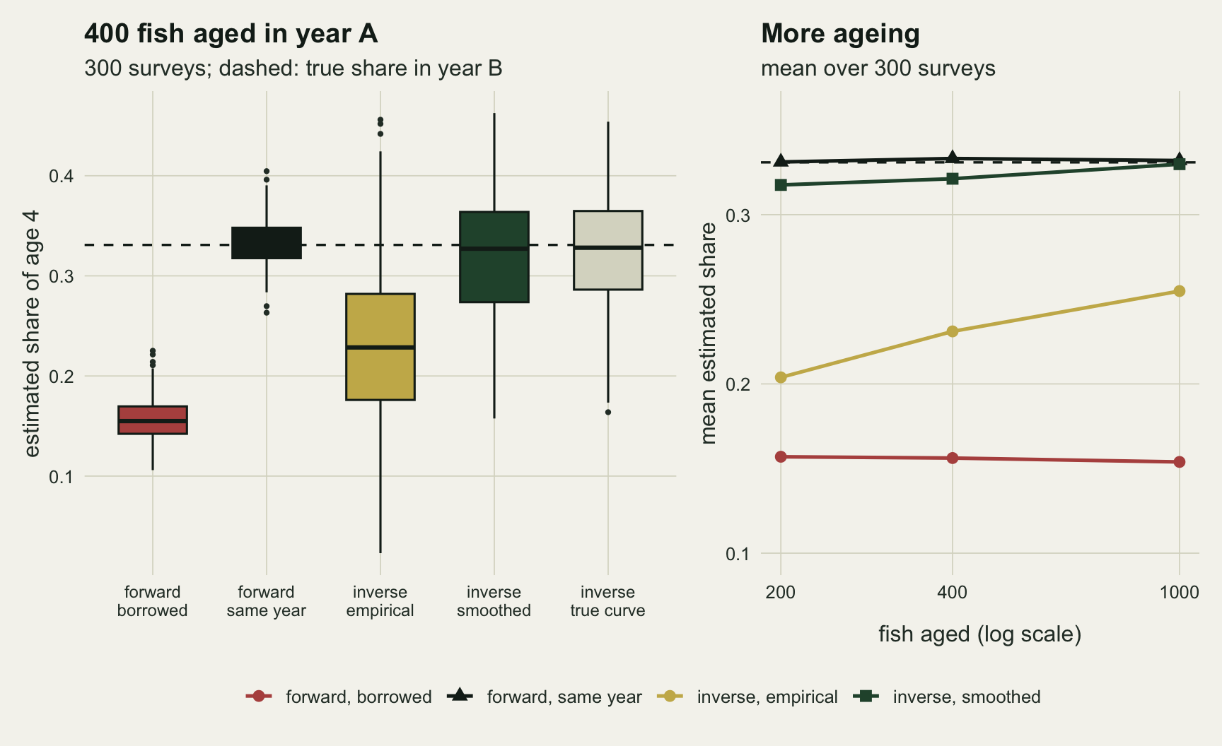
Where the empirical inverse key loses the strong class
Two explanations were on the table for the empirical key’s shortfall. One is that the reported proportions are not the maximum of the likelihood, which is the standing risk with EM on overlapping components. The other is that the key’s length distribution for each age is built from few fish: with 400 aged fish, age 4 is expected to contribute 44 of them, spread over about 10 length bins that cover four standard deviations.
fit_check <- function(cells) {
  fl <- unlist(lapply(cells, function(cc) cc$fits), recursive = FALSE)
  c(fits = sum(sapply(fl, function(f) length(f$gap))),
    capped = sum(sapply(fl, function(f) sum(f$capped))),
    over = sum(sapply(fl, function(f) sum(f$gap > gap_tol))))
}
chk_main <- fit_check(main_cells)

rid_all <- rep(seq_len(n_rep_main), each = n_bin)
q_em <- matrix(1 / n_age, n_rep_main, n_age)
for (it in 1:3000) q_em <- em_step(q_em, c400$p_emp, c400$counts, rid_all)
em_gap <- max(abs(q_em[, strong_use] - c400$share[, "empirical"]))
gap_frac  <- c400$gap_share
zero_part <- gap_frac * share_true / (share_true - s_emp["mean"])
The first explanation fails. Of the 2100 inverse-key fits in the surveys above, 20 stopped at the limit of 200 Newton steps and 8 ended further than 0.00001 from the maximum, so the shares reported in this post are the maxima themselves. For the 300 empirical keys at 400 aged fish, 3000 plain EM steps from equal proportions give an age 4 share within 1.4e-04 of that maximum in every survey. The shortfall belongs to the estimator, not to the algorithm.
The sparse cells are the answer, and it is the thin cells more than the empty ones. In a typical survey only 0.060 of year B’s age 4 fish fall into a length bin where the aged sample holds no age 4 fish at all. Even if every one of those fish were lost to other ages, that would be 0.20 of the shortfall. The rest is consistent with jagged occupied cells: a year B fish in a bin where the age 4 histogram happens to dip is handed to age 3 or age 5 where their histograms happen to peak, and the strong class has the most fish to lose. The smoothed key replaces the jagged histogram with a curve that borrows strength across ages, and it removes 90 per cent of the empirical key’s remaining bias.
Older classes overlap, and there a model does not save it
The headline case put the strong class at age 4. The same design was repeated with the class at age 2, 4 or 6 and a strength of 2, 4 or 8, with 400 aged fish and 100 surveys in each new cell.
grid_cells_def <- expand.grid(strong_age = c(2, 4, 6), strength = c(2, 4, 8))
grid_cells_def <- grid_cells_def[!(grid_cells_def$strong_age == strong_use & grid_cells_def$strength == mult_use), ]
set.seed(6121)
grid_cells <- lapply(seq_len(nrow(grid_cells_def)), function(i)
  run_cell(n_rep_grid, 400, grid_cells_def$strong_age[i], grid_cells_def$strength[i],
           c("forward", "empirical", "smoothed", "truecurve")))
grid_cells <- c(grid_cells, list(c400))
grid_tab <- do.call(rbind, lapply(grid_cells, function(cc) {
  data.frame(strong_age = cc$strong_age, strength = cc$strength,
             arm = c("forward", "empirical", "smoothed", "truecurve"),
             ratio = colMeans(cc$share[, c("forward", "empirical", "smoothed", "truecurve")]) / cc$true_share,
             se = apply(cc$share[, c("forward", "empirical", "smoothed", "truecurve")], 2, sd) /
               sqrt(nrow(cc$share)) / cc$true_share)
}))
gr <- function(sa, st, arm) grid_tab$ratio[grid_tab$strong_age == sa & grid_tab$strength == st & grid_tab$arm == arm]
true6_range <- range(grid_tab$ratio[grid_tab$strong_age == 6 & grid_tab$arm == "truecurve"])
true24_range <- range(grid_tab$ratio[grid_tab$strong_age != 6 & grid_tab$arm == "truecurve"])

cell68  <- grid_cells[[which(grid_cells_def$strong_age == 6 & grid_cells_def$strength == 8)]]
share68 <- cell68$share[, "truecurve"]
pb68    <- year_b_props(6, 8)
ml_expected <- mix_mle(len_given_age, as.vector(len_given_age %*% pb68) * n_meas)$q[6]
true6_row <- grid_tab[grid_tab$strong_age == 6 & grid_tab$arm == "truecurve", ]
true6_se  <- true6_row$se[which.max(true6_row$ratio)]
chk_grid <- fit_check(grid_cells[-length(grid_cells)])
At age 2 every inverse key is close to the truth: the true-curve key’s ratio is 1.001 and the empirical key’s 0.975 at eight times the normal strength. At age 4 the growth curve is what brings the inverse key back, as above. At age 6 the picture changes. Even the control with the true length distributions reaches only 0.80 to 0.91 of the true share across the three strengths, where at ages 2 and 4 it reached 0.98 to 1.00. The smoothed key sits below the control again, at 0.746, 0.801 and 0.784, and the empirical key falls to 0.373 at eight times the normal strength, not far above the borrowed forward key at 0.297.
All 2400 new fits in the grid passed the same check (11 at the step limit, 2 beyond the bound). The part of that residual the control shares is neither a sparse cell nor the growth model. Fed the exact expected length frequency of the age 6, eight-fold case, the same likelihood returns an age 6 share of 0.3162 against the true 0.3162, so the estimator is consistent. With 2000 random lengths the maxima average 0.268: the shortfall is a finite-sample property of separating heavily overlapping components from lengths alone.
grid_plot <- grid_tab
grid_plot$arm <- factor(arm_lab[grid_plot$arm], levels = arm_lab[c(1, 3, 4, 5)])
grid_plot$age_lab <- factor(paste("strong class at age", grid_plot$strong_age))
grid_cols <- arm_cols
grid_cols["inverse, true curve"] <- te_ink
ggplot(grid_plot, aes(strength, ratio, colour = arm)) +
  geom_hline(yintercept = 1, linetype = "dashed", colour = te_body, linewidth = 0.5) +
  geom_errorbar(aes(ymin = ratio - 2 * se, ymax = ratio + 2 * se), width = 0.06, linewidth = 0.5,
                position = position_dodge(width = 0.09)) +
  geom_line(linewidth = 0.8, position = position_dodge(width = 0.09)) +
  geom_point(size = 2, position = position_dodge(width = 0.09)) +
  facet_wrap(~ age_lab) +
  scale_colour_manual(values = grid_cols, name = NULL) +
  scale_x_log10(breaks = c(2, 4, 8)) +
  scale_y_continuous(limits = c(0, 1.15), breaks = seq(0, 1, by = 0.25)) +
  labs(x = "strength of the year class (times its even-recruitment share)",
       y = "estimated share / true share",
       title = "Older classes overlap in length, and every inverse key falls short there",
       subtitle = "400 fish aged in year A, 2000 measured in year B; bars: two Monte Carlo SE") +
  theme_datasheet() + theme(legend.position = "bottom")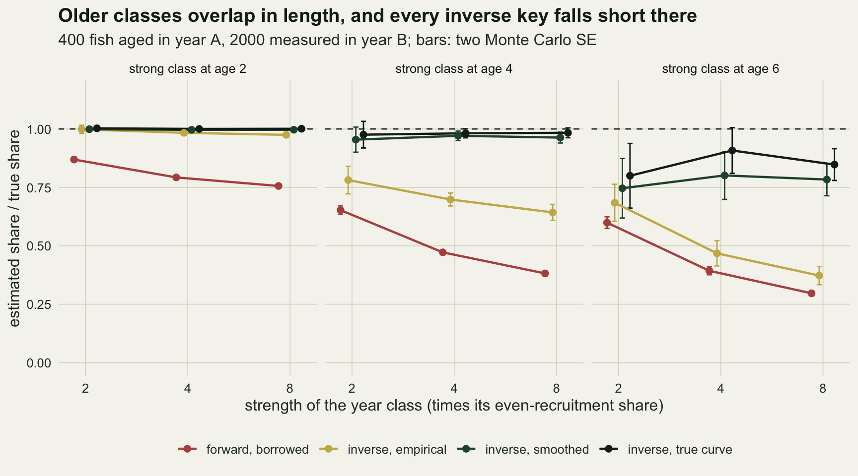
What the catch curve sees
Age compositions are usually wanted for mortality. Each estimated composition was turned into counts at age and a catch curve was fitted as a Poisson log-linear regression of count on age, over all eight ages, since the simulated gear catches every age alike.
z_expected <- function(p_vec) catch_curve_z(p_vec * n_meas)
z_cells <- do.call(rbind, lapply(grid_cells, function(cc) {
  zm <- colMeans(cc$z_hat)
  data.frame(strong_age = cc$strong_age, strength = cc$strength,
             truth = zm["truth"], forward = zm["forward"], empirical = zm["empirical"],
             smoothed = zm["smoothed"])
}))
z_even <- z_expected(prop_a)
key_shift <- with(z_cells, pmax(abs(forward - truth), abs(empirical - truth), abs(smoothed - truth)))
class_shift <- abs(z_cells$truth - z_mort)
z_row <- function(sa, st) z_cells[z_cells$strong_age == sa & z_cells$strength == st, ]
z44 <- z_row(4, 4); z68 <- z_row(6, 8)
max_key_shift <- max(key_shift)
shift_ratio_max <- max(key_shift / class_shift)
In year A the catch curve returns the mortality exactly, 0.35. A strong class breaks the constant-recruitment assumption before any key is involved: with the true year B ages the catch curve gives 0.278 for the age 4, four-fold case and 0.149 for an eight-fold class at age 6. Across all nine cells the largest shift any key makes relative to the true-age catch curve is 0.042, at most 0.28 of the shift the year class itself makes, and the direction is not fixed: in the age 6, eight-fold case the borrowed key gives 0.185, nearer the real mortality than the true ages, because it flattens the class that bends the curve. The borrowed key does its damage to the age composition and to anything that tracks a year class, not to a single catch curve.
What to report
State where the key came from: the year, the survey or the region of the aged fish, and the year of the length frequency it was applied to. If they differ, the estimate carries the age structure of the key’s year, and the matrix product in the section on the borrowed key gives the expected bias for any assumed pair of age structures in a few lines. A strong year class moving through the data is exactly the case where that assumption fails, and the survey that has just found one is the survey most tempted to borrow a key.
If a same-year key is impossible, use an inverse key with a fitted growth curve rather than the raw length-at-age proportions, and report its standard error. In this simulation the smoothed inverse key recovered 0.971 of the age 4 share with a standard deviation 2.7 times that of a same-year key; a borrowed key would look precise and be wrong. Say which ages are well separated in length. For classes whose length distributions overlap as much as ages 5 and 6 do here, no inverse key recovered the strong class on average from 2000 lengths, not even one given the true growth curve (at most 0.91 of the share at age 6, with a Monte Carlo standard error of 0.05 in that cell; a finite-sample shortfall rather than a biased likelihood), and the honest output is a pooled plus group or an explicit statement that the class strength is not estimable from that year’s lengths.
Treat the catch curve separately. No key moved the catch-curve mortality by more than 0.042 here, while the year class itself moved it by far more. If mortality is the target, the recruitment variation needs dealing with first.
Honest limits
Growth is identical in the two years, length at age is normal with a constant coefficient of variation, and the smoothed key is fitted with that exact model. That is the most favourable case for the smoothed inverse key: faster growth in one year changes the length-given-age table and breaks the inverse key as well, and a misspecified growth model would add its own bias.
The aged fish in year A are a simple random sample. Real programmes age fixed numbers per length class, which leaves the forward key unbiased within a year but means the inverse key needs its length-given-age table weighted back to the population. Re-estimating that table from the unaged lengths as well, as in the joint likelihood of Hoenig and Heisey, was not simulated as an arm. Ages are read without error, selectivity is flat and there is no plus group; ageing error would add to every shortfall above, and dome-shaped selectivity would change the catch-curve section entirely.
The grid is small, with 100 surveys per new cell, so its Monte Carlo standard errors reach 0.069 of the true share at age 6 and the ordering of the smoothed and control arms there is not resolved. Only one strong class was present at a time and year A was perfectly even; a key from a year with its own strong class pulls the composition toward that class, and the matrix product handles that case with no new code.
References
Westrheim SJ, Ricker WE 1978 Journal of the Fisheries Research Board of Canada 35(2):184-189 (10.1139/f78-030)
Kimura DK, Chikuni S 1987 Biometrics 43(1):23-35 (10.2307/2531945)
Hoenig JM, Heisey DM 1987 Transactions of the American Fisheries Society 116(2):232-243 (10.1577/1548-8659(1987)116<232:UOALMW>2.0.CO;2)
Gerritsen HD, McGrath D, Lordan C 2006 ICES Journal of Marine Science 63(6):1096-1100 (10.1016/j.icesjms.2006.04.008)