Zero-inflated and hurdle models for ecological counts

Excess zeros in ecological count data: telling overdispersion apart from zero inflation, then fitting zero-inflated negative binomial and hurdle models in R with pscl. A community ecology tutorial.

Ecological count data are full of zeros. A pitfall trap catches nothing in most plots; a target plant is absent from two thirds of quadrats; a bird is detected at a handful of points and nowhere else. A reasonable first reaction is to reach for a “zero-inflated” model, and a great deal of ecology does exactly that. But excess zeros and a zero-inflated process are not the same thing, and conflating them leads to models that fit no better and read worse.

This post separates two issues that often arrive together. The first is overdispersion, which the count-data post handled by moving from Poisson to a negative binomial. The second is zero inflation, where a separate process generates “extra” zeros on top of whatever the count distribution already produces. We build data with a genuine structural-zero process, show why a plain Poisson cannot cope, show the more interesting fact that a negative binomial already absorbs most of the zeros, and then fit the two standard remedies, zero-inflated and hurdle models, with the pscl package. The interpretation of their two halves is where most of the confusion lives, so we spend time there.

Two processes, two kinds of zero

The scenario: a focal species is surveyed across 200 plots. Two things drive what we count. Some plots are simply unsuitable, a dry, bare microhabitat where the species is structurally absent regardless of anything else; the rest are suitable, and there abundance varies with shrub cover. That gives two routes to a zero. A plot can be a structural zero (unsuitable), or it can be a sampling zero, suitable but with a count that happened to land on zero. The distinction is the whole point: only the first is “extra” relative to the count distribution.

library(pscl)
library(MASS)
library(ggplot2)
library(dplyr)
library(tidyr)

set.seed(2025)
n     <- 200
shrub <- runif(n, 0, 1)   # shrub cover, drives abundance where suitable
bare  <- runif(n, 0, 1)   # bare ground, drives structural absence

# structural-zero process: more bare ground, more likely unsuitable
psi    <- plogis(-1.1 + 2.6 * bare)
struct <- rbinom(n, 1, psi)         # 1 = structural zero (unsuitable plot)

# count process where suitable: negative binomial, size = 2
mu    <- exp(0.5 + 2.2 * shrub)
y_pos <- rnbinom(n, mu = mu, size = 2)

# observed count: forced to zero where structurally absent
y   <- ifelse(struct == 1, 0L, y_pos)
dat <- data.frame(y = y, shrub = shrub, bare = bare)

c(zeros = sum(y == 0), pct_zero = round(mean(y == 0), 3), max = max(y))

   zeros pct_zero      max 
 109.000    0.545   30.000 

About 55% of plots hold a zero. Underneath, most of those are structural (the unsuitable plots); a smaller share are sampling zeros from suitable plots whose count fell to zero. In real data we never get to see that split directly, which is exactly why the modelling matters.

Why the Poisson chokes on the zeros

Fit a Poisson and a negative binomial on shrub cover, then ask each model how many zeros it expects. The clean check is to sum each plot’s fitted probability of a zero and compare the total to what we observed.

m_pois <- glm(y ~ shrub, data = dat, family = poisson)
m_nb   <- glm.nb(y ~ shrub, data = dat)

# expected number of zeros under each model
ez_pois <- sum(dpois(0, fitted(m_pois)))
mu_nb   <- fitted(m_nb); th <- m_nb$theta
ez_nb   <- sum((th / (th + mu_nb))^th)

data.frame(
  source   = c("observed", "Poisson", "negative binomial"),
  zeros    = round(c(sum(y == 0), ez_pois, ez_nb), 1)
)

             source zeros
1          observed 109.0
2           Poisson  23.0
3 negative binomial 104.1

The Poisson is hopeless here: it expects roughly 23 zeros against the 109 we saw, a deficit of about 86 plots. That is the textbook signature of “too many zeros”. The negative binomial, though, tells a more subtle story. Its heavier tail piles extra probability near zero, and it ends up expecting around 104 zeros, almost all of them. The deficit has nearly vanished, and we have not written a single line about zero inflation.

This is the point Warton (2005) made directly: many zeros do not mean zero inflation. A long-tailed count distribution produces plenty of zeros on its own, and the bare zero count is not evidence for a separate process. Zero inflation is always defined relative to a model, so the question is never “are there many zeros” but “are there more zeros than this model can produce”.

Looking at the whole shape, not just the zeros

If the negative binomial already covers the zeros, why bother with anything else? Because the price it pays shows up just next door. To manufacture enough zeros from a single count distribution, the negative binomial has to bend its whole low end, and it over-predicts the ones. Comparing the observed count frequencies to the fitted frequencies makes this visible.

m_zinb <- zeroinfl(y ~ shrub | bare, data = dat, dist = "negbin")

maxc <- 8
obs  <- sapply(0:maxc, function(k) sum(y == k))
enb  <- sapply(0:maxc, function(k)
           sum((th/(th+mu_nb))^th * choose(k+th-1, k) * (mu_nb/(mu_nb+th))^k))
ppz  <- predict(m_zinb, type = "prob")
ezi  <- sapply(0:maxc, function(k) sum(ppz[, as.character(k)]))

freq <- data.frame(count = 0:maxc, Observed = obs,
                   `Negative binomial` = enb, `Zero-inflated NB` = ezi,
                   check.names = FALSE) |>
  pivot_longer(-count, names_to = "src", values_to = "freq") |>
  mutate(src = factor(src, levels = c("Observed","Negative binomial","Zero-inflated NB")))

ggplot(freq, aes(count, freq, fill = src)) +
  geom_col(position = position_dodge(width = 0.8), width = 0.75) +
  scale_fill_manual(values = c("Observed"="#16241d",
                               "Negative binomial"="#b5534e",
                               "Zero-inflated NB"="#2f8f63")) +
  scale_x_continuous(breaks = 0:maxc) +
  labs(x = "Count", y = "Number of plots", fill = NULL) +
  theme_minimal(base_size = 12) +
  theme(panel.grid.minor = element_blank(), legend.position = "top")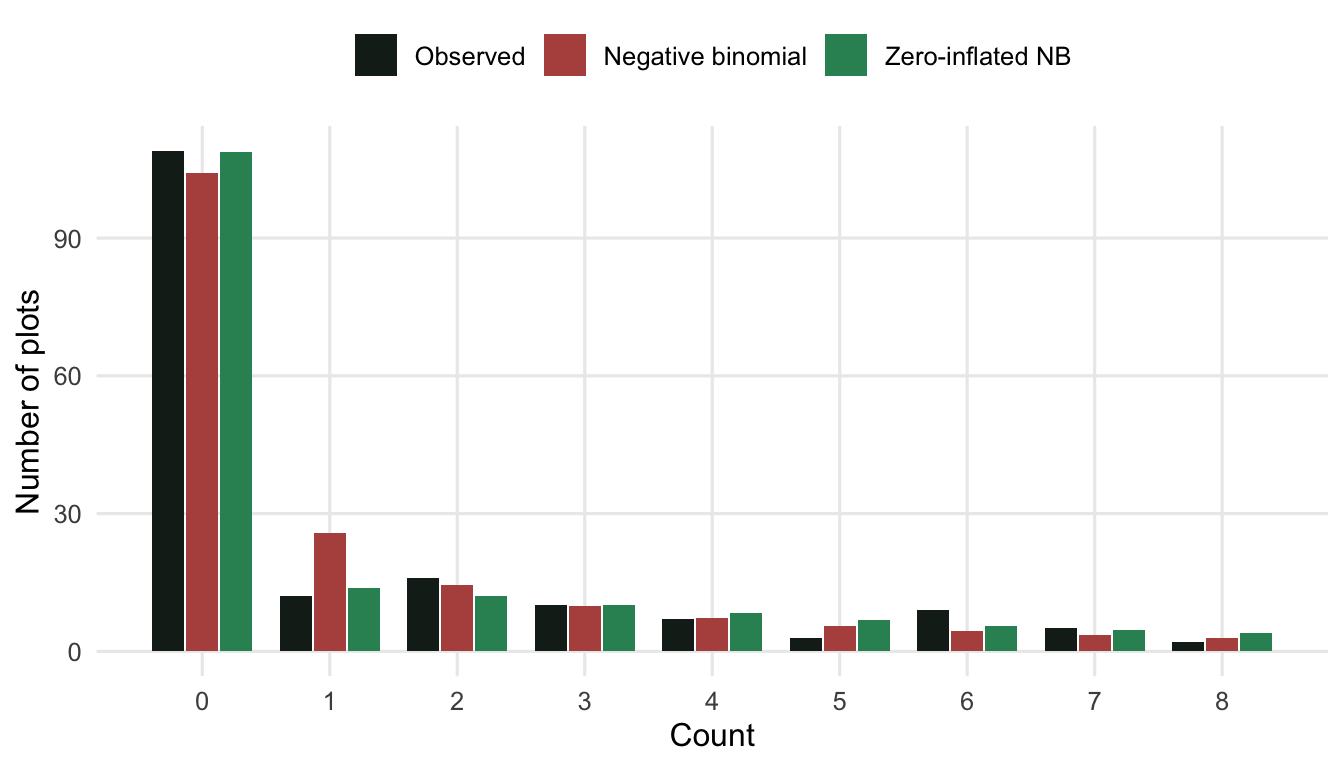

Figure 1

At a count of zero the observed bar and the zero-inflated bar sit together near 109, with the negative binomial a touch short. The tell is at a count of one: the negative binomial expects about 26 plots there, more than double the 12 we actually saw, because that is the cost of stretching one distribution to cover the zeros. The zero-inflated model keeps the zeros and the ones both in line, because it does not have to compromise: a dedicated component handles the structural zeros and frees the count component to fit the suitable plots honestly.

The zero-inflated negative binomial

A zero-inflated model is a mixture. With some probability a plot is a structural zero; otherwise its count comes from a negative binomial that can itself produce zeros. In pscl, the formula y ~ shrub | bare reads as “count model on the left of the bar, zero-inflation model on the right”, so abundance depends on shrub cover while the structural-zero probability depends on bare ground.

summary(m_zinb)$coefficients

$count
             Estimate Std. Error  z value     Pr(>|z|)
(Intercept) 0.4699726  0.2362076 1.989659 4.662854e-02
shrub       2.2338230  0.3551664 6.289512 3.184659e-10
Log(theta)  0.4606230  0.2645574 1.741108 8.166462e-02

$zero
             Estimate Std. Error   z value     Pr(>|z|)
(Intercept) -1.371950  0.4069597 -3.371217 7.483677e-04
bare         2.521971  0.6367334  3.960795 7.470069e-05

The count component recovers the truth well: a strong positive shrub effect, and a dispersion close to what we built in. On the response scale the shrub slope means abundance multiplies by roughly nine across the full range of shrub cover. The zero-inflation component shows a clear positive effect of bare ground on the odds of a structural zero, around a twelvefold increase in those odds from no bare ground to full bare ground. Both halves point where they should.

A useful way to read a zero-inflated fit is to separate the count the species would reach if a plot were suitable from the count we actually expect once the chance of structural absence is folded in.

b <- coef(m_zinb)
nd <- data.frame(shrub = seq(0, 1, length.out = 60))
cnt   <- exp(b["count_(Intercept)"] + b["count_shrub"] * nd$shrub)
pzero <- plogis(b["zero_(Intercept)"] + b["zero_bare"] * mean(dat$bare))
overall <- cnt * (1 - pzero)

curves <- data.frame(shrub = nd$shrub,
                     `Count component (if suitable)` = cnt,
                     `Overall expected count` = overall,
                     check.names = FALSE) |>
  pivot_longer(-shrub, names_to = "which", values_to = "pred")

ggplot() +
  geom_point(data = dat, aes(shrub, y), colour = "#275139", alpha = 0.35, size = 1.4) +
  geom_line(data = curves, aes(shrub, pred, colour = which, linetype = which),
            linewidth = 1) +
  scale_colour_manual(values = c("Count component (if suitable)"="#b5534e",
                                 "Overall expected count"="#2f8f63")) +
  scale_linetype_manual(values = c("Count component (if suitable)"="dashed",
                                   "Overall expected count"="solid")) +
  labs(x = "Shrub cover", y = "Count", colour = NULL, linetype = NULL) +
  theme_minimal(base_size = 12) +
  theme(panel.grid.minor = element_blank(), legend.position = "top")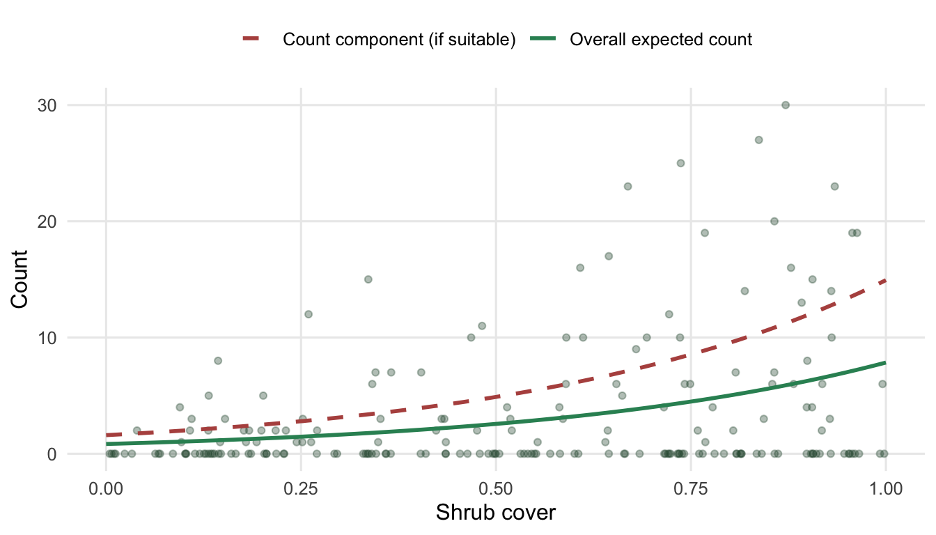

Figure 2

The gap between the dashed and solid curves is the zero-inflation effect made concrete: the species can reach high abundance where conditions allow, but the constant risk that a plot is unsuitable pulls the population-level expectation down across the board.

The hurdle alternative, and a sign that trips everyone up

A hurdle model splits the data differently. It is a two-part model: a binomial model for whether the count clears zero at all, then a zero-truncated count model for the positive values. Where the zero-inflated model lets zeros arrive from two sources, the hurdle insists that every zero is a “below the hurdle” zero, and every positive count comes from a distribution that cannot itself be zero. For abundance data with a clean presence step, that often reads more naturally.

m_hur <- hurdle(y ~ shrub | bare, data = dat, dist = "negbin")
summary(m_hur)$coefficients

$count
             Estimate Std. Error  z value     Pr(>|z|)
(Intercept) 0.5061569  0.2504085 2.021325 4.324615e-02
shrub       2.1803471  0.3704955 5.884949 3.981773e-09
Log(theta)  0.4683368  0.2706443 1.730452 8.354962e-02

$zero
              Estimate Std. Error   z value    Pr(>|z|)
(Intercept)  0.8874636  0.2943225  3.015275 0.002567460
bare        -2.1522904  0.5185893 -4.150279 0.000033207

The count halves of the two models agree almost exactly, which is reassuring. The zero halves look like they disagree, and this is the single most common misreading of these models. The bare-ground coefficient is positive in the zero-inflated model and negative in the hurdle, and nothing is wrong. The two halves model opposite events. The zero-inflation component predicts the probability of a structural zero, so more bare ground raises it. The hurdle’s binomial component predicts the probability of clearing the hurdle, that is of being present, so more bare ground lowers it. Same data, same direction of the underlying ecology, opposite-signed coefficients, purely because the two parameterisations point their zero models at mirror-image outcomes. Always check which event the zero model is describing before you read its sign.

Choosing, and the deeper question

By AIC the ordering is unambiguous: the Poisson is far behind, the negative binomial is a large improvement, and the zero-inflated and hurdle models edge ahead of it and sit close to each other.

AIC(m_pois, m_nb, m_zinb, m_hur)

       df       AIC
m_pois  2 1626.5259
m_nb    3  797.4948
m_zinb  5  760.2380
m_hur   5  763.3848

It is tempting to settle the zero-inflated-versus-not question with a Vuong test, and pscl will compute one. We do not lean on it here. Wilson (2015) showed that a zero-inflated model and its plain counterpart do not meet the conditions the Vuong test assumes for non-nested models, so its use for exactly this comparison is not valid, and it can behave erratically. Information criteria, or honest out-of-sample comparison, are the safer ground.

The more important point is that the choice is mechanistic before it is statistical. Martin et al. (2005) framed it as asking where a zero came from, and Blasco-Moreno et al. (2019) sharpened the taxonomy into false zeros (an observer or design error), sampling zeros (the species was there but went undetected or simply was not counted), and structural zeros (the species cannot occur there). A hurdle suits a clean presence-then-abundance story. A zero-inflated model suits the case where suitable plots can still read zero and you want to keep those zeros inside the count process. And when a negative binomial already covers the zeros, as it nearly did here, the most defensible move may be to add no zero component at all, and to say so.

Takeaways

Excess zeros are a property of the data relative to a model, not a property of the data alone; the negative binomial often soaks up most of them through its tail (Warton 2005). When a separate absence process is real, a zero-inflated model treats zeros as a mixture and a hurdle treats them as a two-part presence step, and the two count halves usually agree. The zero halves can carry opposite signs because they describe opposite events, so read them by their target, not their sign. Prefer information criteria to the Vuong test for the zero-inflation comparison (Wilson 2015), and decide on the model from where you think the zeros came (Martin et al. 2005; Blasco-Moreno et al. 2019), not from a reflex.

A related strand on non-independence in ecological models, where ignoring structure inflates confidence rather than zeros, runs through the spatial autocorrelation post.

References

Blasco-Moreno, A., Perez-Casany, M., Puig, P., Morante, M. & Castells, E. (2019). What does a zero mean? Understanding false, random and structural zeros in ecology. Methods in Ecology and Evolution, 10(7), 949-959. https://doi.org/10.1111/2041-210X.13185

Lambert, D. (1992). Zero-inflated Poisson regression, with an application to defects in manufacturing. Technometrics, 34(1), 1-14. https://doi.org/10.2307/1269547

Martin, T. G., Wintle, B. A., Rhodes, J. R., Kuhnert, P. M., Field, S. A., Low-Choy, S. J., Tyre, A. J. & Possingham, H. P. (2005). Zero tolerance ecology: improving ecological inference by modelling the source of zero observations. Ecology Letters, 8(11), 1235-1246. https://doi.org/10.1111/j.1461-0248.2005.00826.x

Mullahy, J. (1986). Specification and testing of some modified count data models. Journal of Econometrics, 33(3), 341-365. https://doi.org/10.1016/0304-4076(86)90002-3

Warton, D. I. (2005). Many zeros does not mean zero inflation: comparing the goodness-of-fit of parametric models to multivariate abundance data. Environmetrics, 16(3), 275-289. https://doi.org/10.1002/env.702

Wilson, P. (2015). The misuse of the Vuong test for non-nested models to test for zero-inflation. Economics Letters, 127, 51-53. https://doi.org/10.1016/j.econlet.2014.12.029

Zeileis, A., Kleiber, C. & Jackman, S. (2008). Regression models for count data in R. Journal of Statistical Software, 27(8), 1-25. https://doi.org/10.18637/jss.v027.i08