library(ggplot2)

te_pal <- list(forest = "#275139", green = "#2f8f63", sage = "#93a87f",
               clay = "#b5534e", gold = "#cda23f", line = "#dad9ca",
               ink = "#16241d", paper = "#f5f4ee")

theme_te <- function() {
  theme_minimal(base_size = 12) +
    theme(panel.grid.minor = element_blank(),
          panel.grid.major = element_line(colour = "#e7e6dc"),
          plot.background = element_rect(fill = "#f5f4ee", colour = NA),
          panel.background = element_rect(fill = "#f5f4ee", colour = NA),
          plot.title = element_text(face = "bold", colour = te_pal$ink),
          axis.title = element_text(colour = "#2c3a31"),
          axis.text = element_text(colour = "#2c3a31"))
}Parasite burdens truncated by host death
R
parasitology
count data
selection bias
ecology tutorial
Hosts carrying the heaviest worm burdens die before the survey reaches them. Simulating that truncation in R and measuring what it does to the mean and to k.
Two hundred and forty wood mice, trapped at eight woodland sites over three autumns, dissected one at a time, with the small intestine opened under a scope and every adult nematode counted. The number that goes into the spreadsheet is one integer per mouse. About a quarter of the mice carry nothing at all. Most of the rest carry a handful. Four or five carry more worms between them than the whole bottom half put together.
That shape is the oldest quantitative fact in parasitology. Crofton (1971) set it out as the defining property of parasitism: hosts do not share their parasites evenly, and the distribution of burdens across a host population is overdispersed by a wide margin relative to a Poisson. The negative binomial with a small aggregation parameter \(k\) is the standard description, and Shaw and Dobson (1995) found small values of \(k\) across a large collection of published wildlife datasets. Shaw, Grenfell and Dobson (1998) went further and asked which aggregated family fits best; the negative binomial won often enough to remain the default.
The difficulty is in the same sentence as the finding. A mouse carrying two hundred worms is a mouse in trouble. Heavy burdens damage the gut wall, cost the host protein it cannot spare, slow it down, and make it easier to catch. Whatever kills it, the mouse is dead before the trap line goes out, and the count it would have contributed never reaches the spreadsheet. The survey does not sample the burden distribution. It samples the burden distribution of the animals that survived it, which is the same distribution with its upper tail thinned or removed. Crofton (1971) named this in the second of his two papers that year and built a model around it, and Anderson and Gordon (1982) worked out what parasite-induced mortality does to the shape of the observed distribution. Lester (1984) went through the methods a fisheries parasitologist could use to detect the same thing in a wild fish population, and was blunt about how little any of them settle.
This post measures the damage and then measures the repair, and the second measurement is the one that matters. It sits next to four posts and repeats none of them. Poisson and negative binomial GLMs in R fits the negative binomial whose two parameters are the subject here, and takes both of them at face value; this post shows that under truncation one of them is badly wrong and the other is nearly right, which is not the pattern anybody expects. Zero-inflated and hurdle models for ecological counts is the mirror image: extra mass at zero against missing mass in the tail, and both are read off the same dispersion statistic, so the two failures are hard to tell apart from a fitted model alone. Collider bias and selection is the same mechanism written in causal notation, because surviving to be trapped is a common effect of burden and of everything else about the mouse, and conditioning on it is conditioning on a collider. And the abundance-occupancy relationship is the other post on this site that reads the negative binomial \(k\) as a statement about aggregation rather than as a nuisance parameter.
The population, and the part of it that dies
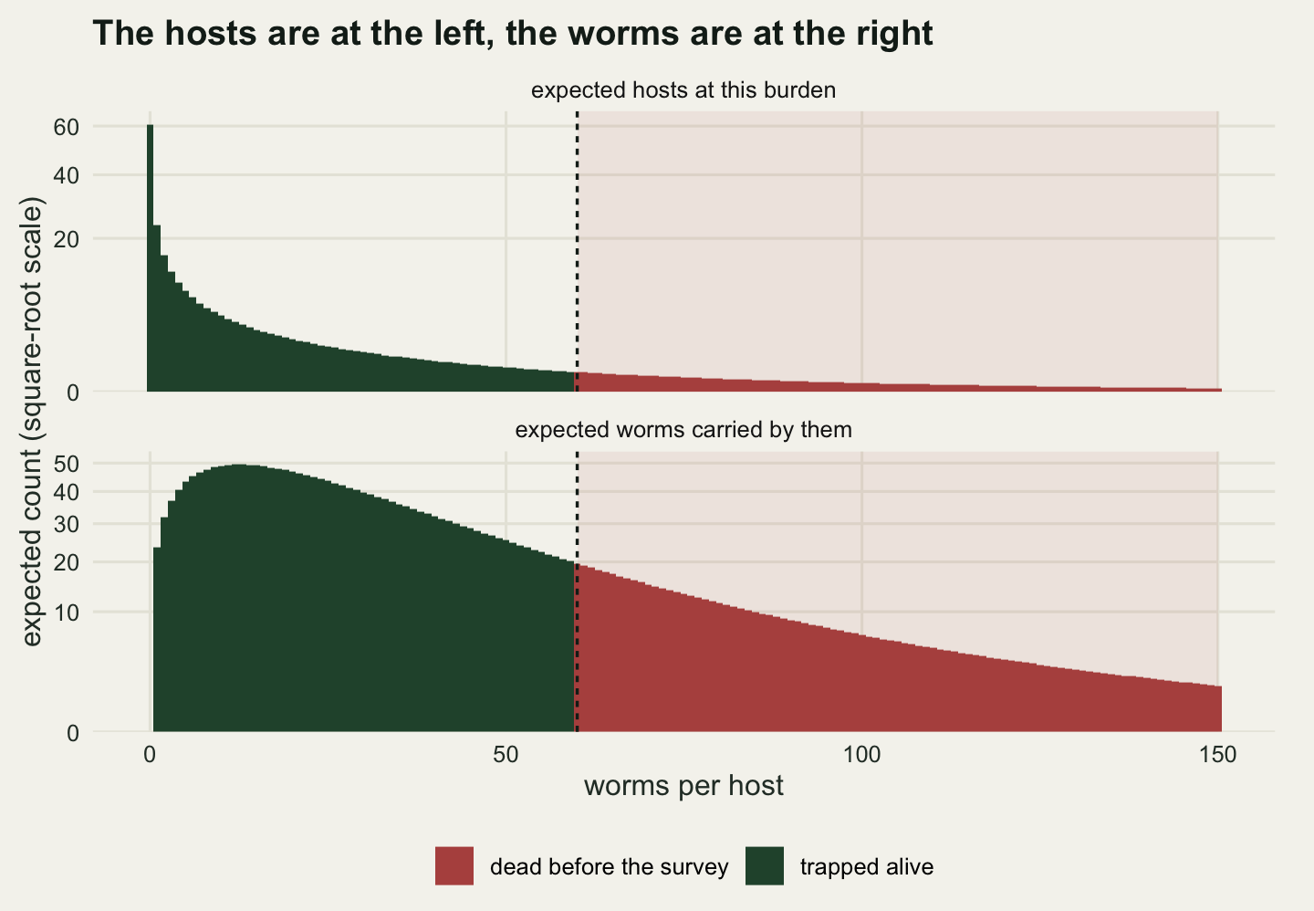
The generating model is a negative binomial with a mean of twelve worms per host and an aggregation parameter of four tenths. Both are ordinary values for a gut nematode in a small mammal. The lethal level is set at sixty worms to begin with: every host above it is dead before the survey, every host below it is available to be trapped. That is a caricature, and the smooth version comes two sections later, but it makes the arithmetic legible.
mu_true <- 12
k_true <- 0.4
lethal <- 60
n_host <- 240

x_grid <- 0:4000
p_true <- dnbinom(x_grid, size = k_true, mu = mu_true)

frac_hosts_lost <- sum(p_true[x_grid >= lethal])
frac_worms_lost <- sum(x_grid * p_true * (x_grid >= lethal)) / mu_true
vmr_true <- 1 + mu_true / k_true
prev_true <- 1 - dnbinom(0, size = k_true, mu = mu_true)

print(round(c(mean_burden = mu_true, k = k_true,
              variance = mu_true + mu_true^2 / k_true,
              variance_to_mean = vmr_true,
              prevalence = prev_true,
              pmf_sums_to = sum(p_true)), 5))
mean_burden k variance variance_to_mean
12.0000 0.4000 372.0000 31.0000
prevalence pmf_sums_to
0.7468 1.0000 print(round(c(lethal_level = lethal,
hosts_at_or_above = frac_hosts_lost,
worms_at_or_above = frac_worms_lost,
hosts_in_survey = n_host), 5)) lethal_level hosts_at_or_above worms_at_or_above hosts_in_survey
60.00000 0.03461 0.24625 240.00000 The population prevalence is 74.68 per cent, so a quarter of the mice are uninfected and the survey would report that correctly. The variance is 372 against a mean of 12, a variance-to-mean ratio of 31, which is what aggregation means in one number.
The two figures that matter are in the second block. The lethal level removes 3.46 per cent of the hosts and 24.63 per cent of the worms. That gap is the whole problem in one line. Losing three hosts in a hundred sounds like nothing. Losing a quarter of the worms is not nothing, and the worms are what the survey exists to count.
Fitting the negative binomial the survey actually has
The likelihood is worth writing out once rather than calling. For a burden \(x\) with mean \(\mu\) and aggregation parameter \(k\), the negative binomial probability is
\[ P(X = x) \;=\; \frac{\Gamma(x + k)}{\Gamma(k)\,x!} \left(\frac{k}{k + \mu}\right)^{\!k} \left(\frac{\mu}{k + \mu}\right)^{\!x} \]
and the log likelihood is the sum of the logarithm of that over the hosts. Everything that follows in this post is a modification of the same three lines, so it pays to see them once.
nb_loglik <- function(x, mu, kk) {
  sum(lgamma(x + kk) - lgamma(kk) - lgamma(x + 1) +
        kk * log(kk / (kk + mu)) + x * log(mu / (kk + mu)))
}

fit_nb <- function(x) {
  opt <- optim(c(log(mean(x) + 0.5), 0),
               function(par) -nb_loglik(x, exp(par[1]), exp(par[2])),
               control = list(reltol = 1e-12, maxit = 5000))
  c(mu = exp(opt$par[1]), k = exp(opt$par[2]), loglik = -opt$value)
}
One survey first. The trapping draws two hundred and forty hosts from the population, the ones at or above the lethal level are removed, and the ordinary negative binomial is fitted to what is left. MASS::glm.nb fits the same likelihood by iterated weighted least squares and is used here only to confirm that the hand-written version has not gone astray.
set.seed(20260804)
burden_all <- rnbinom(n_host, size = k_true, mu = mu_true)
burden_obs <- burden_all[burden_all < lethal]

fit_all <- fit_nb(burden_all)
fit_obs <- fit_nb(burden_obs)
check <- MASS::glm.nb(burden_obs ~ 1)

print(round(c(hosts_dissected = length(burden_obs),
              hosts_lost = n_host - length(burden_obs),
              largest_burden_seen = max(burden_obs),
              zeros = sum(burden_obs == 0),
              sample_mean = mean(burden_obs)), 4))
hosts_dissected hosts_lost largest_burden_seen zeros
230.000 10.000 56.000 57.000
sample_mean
10.187 print(round(rbind(complete_population = fit_all,
survivors_only = fit_obs), 5)) mu k loglik
complete_population 13.80003 0.40399 -824.8045
survivors_only 10.18694 0.46364 -742.8377print(round(c(glm_nb_mu = unname(exp(coef(check))),
glm_nb_k = check$theta,
hand_written_mu = unname(fit_obs["mu"]),
hand_written_k = unname(fit_obs["k"])), 5)) glm_nb_mu glm_nb_k hand_written_mu hand_written_k
10.18696 0.46364 10.18694 0.46364 The two fits of the same likelihood agree to five decimal places, so the hand-written version is doing what it should. On this survey the lethal level removed 10 of the 240 hosts and the largest burden anybody saw was 56 worms. The complete sample would have given a mean of 13.8 and a \(k\) of 0.404. The survivors give a mean of 10.187 and a \(k\) of 0.4636.
One survey settles nothing. The next block runs eight hundred of them, and adds a second, more believable removal rule alongside the hard cut: survival declines smoothly with burden, following a logistic curve with a half-survival point at forty-five worms and a scale of twelve, so a mouse with twenty worms almost always lives, one with forty-five is a coin flip, and one with eighty rarely makes it.
x50 <- 45
s_mort <- 12
host_survival <- function(x) 1 / (1 + exp((x - x50) / s_mort))

print(round(c(survival_at_10 = host_survival(10),
              survival_at_20 = host_survival(20),
              survival_at_45 = host_survival(45),
              survival_at_80 = host_survival(80),
              survival_at_150 = host_survival(150)), 5))
survival_at_10 survival_at_20 survival_at_45 survival_at_80 survival_at_150
0.94866 0.88927 0.50000 0.05134 0.00016 print(round(c(overall_survival = sum(p_true * host_survival(x_grid)),
mean_of_survivors =
sum(x_grid * p_true * host_survival(x_grid)) /
sum(p_true * host_survival(x_grid))), 5)) overall_survival mean_of_survivors
0.88982 7.94803 Under that curve 88.98 per cent of the hosts are still alive at trapping time, which is a heavier loss than the hard cut inflicts, and the mean burden among the survivors is 7.948 worms against a population mean of 12.
n_rep <- 800
top_fifth <- function(x) {
  srt <- sort(x, decreasing = TRUE)
  sum(srt[seq_len(ceiling(0.2 * length(x)))]) / sum(x)
}
gini_index <- function(x) {
  srt <- sort(x)
  nn <- length(srt)
  sum((2 * seq_len(nn) - nn - 1) * srt) / (nn^2 * mean(srt))
}
moment_k <- function(x) mean(x)^2 / (var(x) - mean(x))

summarise_sample <- function(x) {
  fitted_nb <- fit_nb(x)
  pois_ll <- sum(dpois(x, mean(x), log = TRUE))
  c(mu = unname(fitted_nb["mu"]), k = unname(fitted_nb["k"]),
    k_mom = moment_k(x), vmr = var(x) / mean(x),
    top = top_fifth(x), gini = gini_index(x),
    lrt = 2 * (unname(fitted_nb["loglik"]) - pois_ll), n = length(x))
}

set.seed(4242)
rep_out <- vapply(seq_len(n_rep), function(b) {
  x <- rnbinom(n_host, size = k_true, mu = mu_true)
  hard <- x[x < lethal]
  soft <- x[runif(n_host) < host_survival(x)]
  c(complete = summarise_sample(x),
    cut = summarise_sample(hard),
    smooth = summarise_sample(soft))
}, numeric(24))
rep_out <- as.data.frame(t(rep_out))

col_of <- function(which_set, stat) rep_out[[paste0(which_set, ".", stat)]]
avg <- function(which_set, stat) mean(col_of(which_set, stat))

avg_row <- function(key) vapply(c("mu", "k", "k_mom", "vmr", "n"),
                                function(s) avg(key, s), numeric(1))
print(round(rbind(complete = avg_row("complete"), hard_cut = avg_row("cut"),
                  smooth_mortality = avg_row("smooth")), 4))
mu k k_mom vmr n
complete 11.9690 0.4045 0.4157 30.5648 240.0000
hard_cut 9.3742 0.4507 0.5895 17.0006 231.8025
smooth_mortality 7.9602 0.4532 0.5570 15.4789 213.7038mu_shortfall_cut <- 100 * (1 - avg("cut", "mu") / mu_true)
mu_shortfall_soft <- 100 * (1 - avg("smooth", "mu") / mu_true)
k_infl_ml_cut <- avg("cut", "k") / avg("complete", "k")
k_infl_mom_cut <- avg("cut", "k_mom") / avg("complete", "k_mom")
k_infl_ml_soft <- avg("smooth", "k") / avg("complete", "k")
k_infl_mom_soft <- avg("smooth", "k_mom") / avg("complete", "k_mom")
sd_mu_cut <- sd(col_of("cut", "mu"))
print(round(c(mean_shortfall_pct_hard = mu_shortfall_cut,
mean_shortfall_pct_smooth = mu_shortfall_soft,
bias_in_sd_units = (mu_true - avg("cut", "mu")) / sd_mu_cut,
sd_of_mu_hat = sd_mu_cut), 4)) mean_shortfall_pct_hard mean_shortfall_pct_smooth bias_in_sd_units
21.8819 33.6650 3.2791
sd_of_mu_hat
0.8008 print(round(c(k_inflation_ml_hard = k_infl_ml_cut,
k_inflation_moments_hard = k_infl_mom_cut,
k_inflation_ml_smooth = k_infl_ml_soft,
k_inflation_moments_smooth = k_infl_mom_soft), 4)) k_inflation_ml_hard k_inflation_moments_hard
1.1142 1.4183
k_inflation_ml_smooth k_inflation_moments_smooth
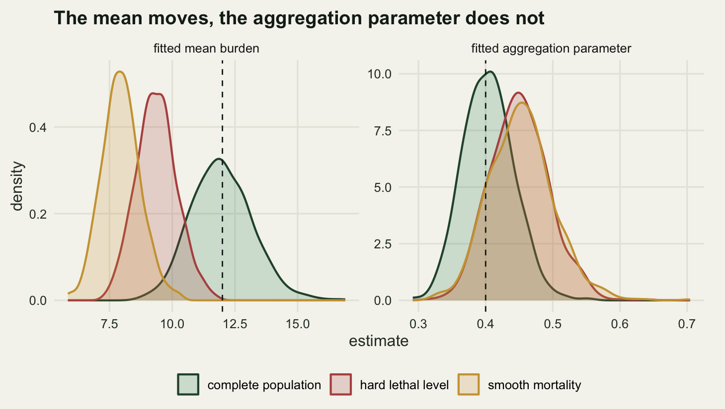
1.1205 1.3400 Over 800 replicates of a 240 host survey, the mean burden comes out 21.88 per cent short under the hard cut and 33.67 per cent short under the smooth mortality curve. The shortfall under the hard cut is 3.28 standard deviations of the estimator, so it is far larger than the sampling noise and every survey is wrong in the same direction; what a single survey cannot do is notice, because it has nothing to compare its answer against.
The aggregation parameter is the surprise, and it went the opposite way to what I expected before running it. The maximum likelihood \(k\) inflates by a factor of 1.114 under the hard cut and 1.12 under smooth mortality: eleven or twelve per cent, not the doubling that the loss of a quarter of the worms suggests. The method-of-moments \(k\), computed from the sample mean and variance and still the estimator behind a great many published aggregation figures, inflates by 1.418 and 1.34. The two estimators of the same parameter disagree by nearly a third on the same data, and only one of them is telling the reader that anything has happened.
The reason is in the likelihood. With \(k\) below one the negative binomial’s shape is set almost entirely by the crowd at the bottom: the height of the zero class relative to the one class relative to the two class. Truncation does not touch any of them. It removes a handful of observations from a region the likelihood was already treating as nearly weightless, and the fitted \(k\) barely moves, while the fitted \(\mu\) moves a long way because the sample mean moved a long way. The moment estimator has no such protection; it is a function of the variance, and the variance is exactly what the missing hosts were carrying.
Aggregation is the finding, and truncation attacks it unevenly
In most other count problems the mean is the answer and the dispersion is a nuisance. In parasitology the dispersion is the answer. Aggregation is what determines whether transmission is sustained by a small subset of hosts, what a mass treatment programme is worth, and whether the parasite regulates the host population at all. Woolhouse and colleagues (1997) put the working version of it in one sentence: for a wide range of infections a fifth of the hosts account for about four fifths of the transmission, and control effort aimed at that fifth buys far more than effort spread evenly. If truncation attacks the aggregation summaries, it attacks the conclusion rather than a detail of it.
Wilson, Grenfell and Shaw (1996) went through the summaries in use and their behaviour. Three of them appear below: the variance-to-mean ratio, the Gini coefficient of the burdens, and the share of the total burden held by the most infected fifth of hosts. The fourth entry is the test that decides whether an aggregated model is needed at all, a likelihood ratio comparison of the fitted negative binomial against a Poisson with the same mean.
agg_tab <- rbind(
  complete = c(vmr = avg("complete", "vmr"), gini = avg("complete", "gini"),
               top_fifth = avg("complete", "top"), lrt = avg("complete", "lrt")),
  hard_cut = c(avg("cut", "vmr"), avg("cut", "gini"),
               avg("cut", "top"), avg("cut", "lrt")),
  smooth_mortality = c(avg("smooth", "vmr"), avg("smooth", "gini"),
                       avg("smooth", "top"), avg("smooth", "lrt")))
print(round(agg_tab, 4))
vmr gini top_fifth lrt
complete 30.5648 0.6868 0.7010 4214.992
hard_cut 17.0006 0.6533 0.6642 2561.595
smooth_mortality 15.4789 0.6584 0.6681 1994.309rel_change <- round(100 * (agg_tab[2:3, 1:3] / rep(agg_tab[1, 1:3], each = 2) - 1), 3)
print(rel_change) vmr gini top_fifth
hard_cut -44.378 -4.882 -5.253
smooth_mortality -49.357 -4.142 -4.696lrt_crit <- qchisq(0.90, 1) # boundary test on 1/k = 0: the null is a 50:50 mixture of
# chi-square on 0 and 1 df, so the 5% point is the 90% point of chi-square(1)
print(round(c(chisq_threshold = lrt_crit,
reject_poisson_complete = mean(col_of("complete", "lrt") > lrt_crit),
reject_poisson_hard = mean(col_of("cut", "lrt") > lrt_crit),
reject_poisson_smooth = mean(col_of("smooth", "lrt") > lrt_crit),
smallest_statistic_hard = min(col_of("cut", "lrt")),
smallest_statistic_smooth = min(col_of("smooth", "lrt"))), 4)) chisq_threshold reject_poisson_complete reject_poisson_hard
2.7055 1.0000 1.0000
reject_poisson_smooth smallest_statistic_hard smallest_statistic_smooth
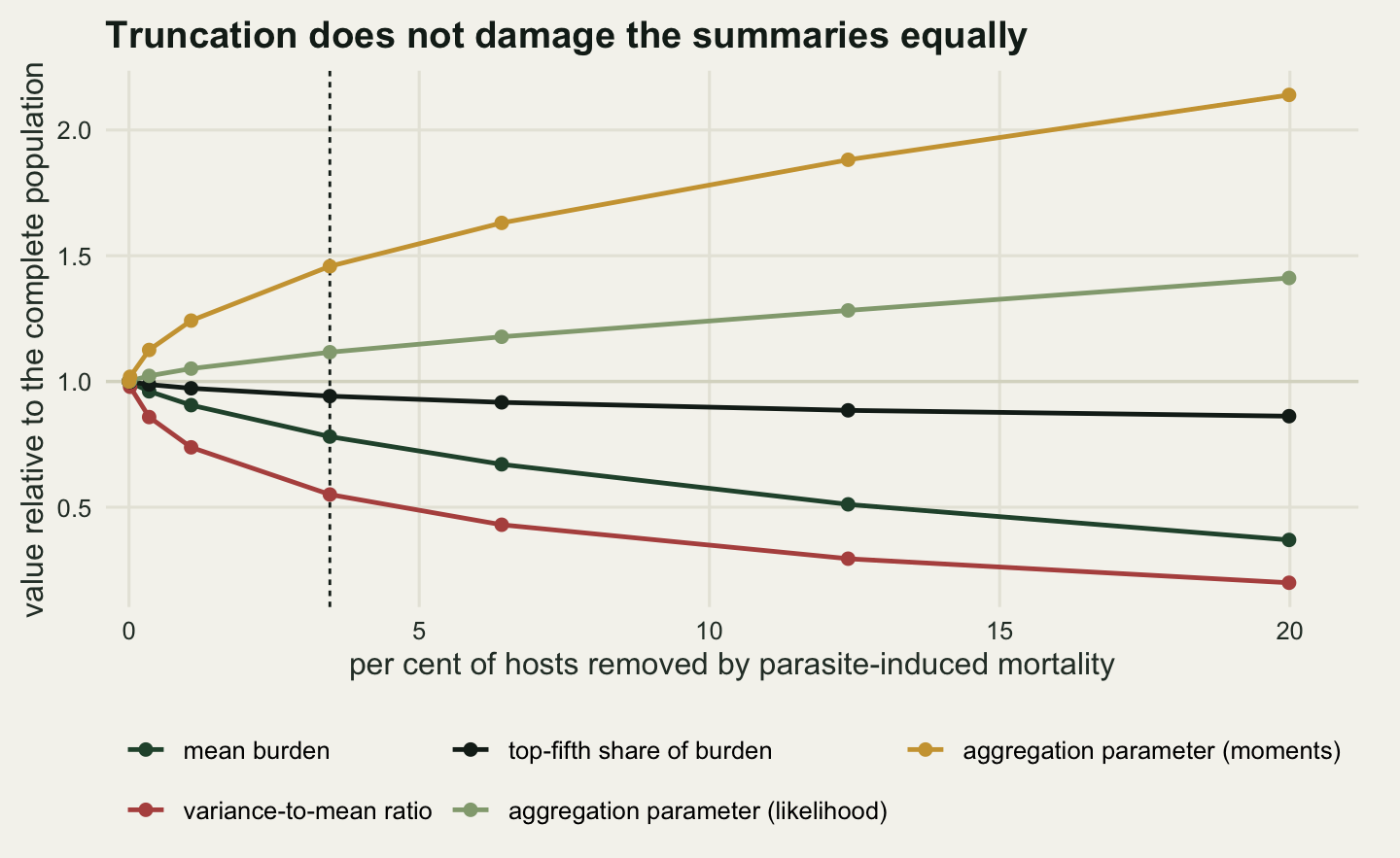
1.0000 1653.9234 1263.4391 The variance-to-mean ratio falls from 30.56 to 17 under the hard cut, a loss of 44.38 per cent of itself, and to 15.48 under smooth mortality. That is the collapse the intuition predicts. The other two summaries do not follow it. The share of the burden held by the top fifth of hosts goes from 0.701 to 0.6642, a fall of 5.25 per cent, and the Gini coefficient falls by 4.88 per cent. A survey that has lost a quarter of its worms still reports that the most infected fifth of hosts carry about two thirds of the burden, because removing the top of the distribution removes it from the numerator and the denominator at once.
The Poisson comparison gives up a good deal of its statistic and none of its verdict. The likelihood ratio statistic averages 2561.6 on the truncated samples, down from 4215 on the complete ones, against a threshold of 2.71, and the smallest value seen across 800 replicates was 1653.9. The Poisson is rejected in every replicate of every version. I expected this one to fail sometimes and it never did at this number of hosts, and the margin is wide enough that it would take a much smaller survey to put the verdict in doubt.
That combination is what lets the problem survive review. A truncated survey still says, correctly, that burdens are aggregated, still reports a top-fifth share close to the truth, and still reports an aggregation parameter only slightly too large. What it gets badly wrong is the mean, and through the mean everything derived from it: the total worm population, the burden of the animals that were not caught, and the variance the fitted model implies, which here is 204.4 against a true 372.
How the damage scales with the severity of the mortality can be had exactly rather than by simulation. The truncated distribution is known in closed form for any lethal level, so each summary follows from it directly, and the value the maximum likelihood fit converges to is the pair minimising the cross entropy between that distribution and the fitted negative binomial. That is the probability limit of the estimator, with no Monte Carlo noise in it.
nb_projection <- function(prob) {
  opt <- optim(c(log(sum(x_grid * prob) + 0.5), 0), function(par) {
    ld <- dnbinom(x_grid, size = exp(par[2]), mu = exp(par[1]), log = TRUE)
    -sum(prob * ifelse(is.finite(ld), ld, -1e6))
  }, control = list(reltol = 1e-14, maxit = 8000))
  c(mu = exp(opt$par[1]), k = exp(opt$par[2]), cross_entropy = -opt$value)
}

top_fifth_exact <- function(prob) {
  tail_p <- rev(cumsum(rev(prob)))
  j <- which(tail_p <= 0.2)[1]
  q <- x_grid[j]
  (sum(x_grid[x_grid >= q] * prob[x_grid >= q]) +
     (0.2 - tail_p[j]) * (q - 1)) / sum(x_grid * prob)
}

summarise_pmf <- function(prob) {
  proj <- nb_projection(prob)
  m <- sum(x_grid * prob)
  v <- sum((x_grid - m)^2 * prob)
  pois_ent <- sum(prob * ifelse(is.finite(dpois(x_grid, m, log = TRUE)),
                                dpois(x_grid, m, log = TRUE), -1e6))
  c(mean = m, vmr = v / m, k_ml = unname(proj["k"]), k_mom = m^2 / (v - m),
    top_fifth = top_fifth_exact(prob),
    deviance_per_host = 2 * (unname(proj["cross_entropy"]) - pois_ent))
}

lethal_grid <- c(400, 200, 120, 90, 60, 45, 30, 20)
sweep_tab <- t(vapply(lethal_grid, function(L) {
  prob <- p_true * (x_grid < L)
  c(lethal_level = L, hosts_lost = 1 - sum(prob),
    summarise_pmf(prob / sum(prob)))
}, numeric(8)))
sweep_full <- c(lethal_level = NA, hosts_lost = 0, summarise_pmf(p_true))
print(round(rbind(no_mortality = sweep_full, sweep_tab), 4))
lethal_level hosts_lost mean vmr k_ml k_mom top_fifth
no_mortality NA 0.0000 12.0000 31.0000 0.4000 0.4000 0.7043
400 0.0000 11.9999 30.9975 0.4000 0.4000 0.7043
200 0.0002 11.9582 30.3465 0.4009 0.4075 0.7035
120 0.0035 11.5293 26.6126 0.4089 0.4501 0.6958
90 0.0107 10.8703 22.8800 0.4205 0.4968 0.6852
60 0.0346 9.3692 17.0642 0.4465 0.5832 0.6633
45 0.0642 8.0468 13.3369 0.4711 0.6523 0.6458
30 0.1239 6.1364 9.1531 0.5130 0.7527 0.6235
20 0.1999 4.4378 6.1853 0.5646 0.8558 0.6071
deviance_per_host
no_mortality 17.7651
17.7647
17.5952
16.2113
14.4459
11.1164
8.6556
5.6312
3.3674smooth_row <- summarise_pmf(p_true * host_survival(x_grid) /
sum(p_true * host_survival(x_grid)))
print(round(smooth_row, 4)) mean vmr k_ml k_mom
7.9480 15.5124 0.4492 0.5477
top_fifth deviance_per_host
0.6664 9.3614 At the lethal level used throughout, losing 3.46 per cent of the hosts costs 21.92 per cent of the mean, 44.95 per cent of the variance-to-mean ratio and 5.83 per cent of the top-fifth share, while inflating the maximum likelihood \(k\) by 11.63 per cent and the moment \(k\) by 45.81 per cent. Push the lethal level down to twenty worms, which removes a fifth of all hosts, and the mean has lost 63.02 per cent while the top-fifth share has lost 13.8 per cent. The ordering never changes over the whole sweep.
The last column explains why the Poisson test is useless here. It is the expected likelihood ratio statistic contributed by one host, so the whole survey’s statistic is that number times the sample size. At the lethal level of sixty it is 11.116, and even at a lethal level of twenty it is 3.367. A survey of two hosts would clear the 2.71 threshold on average. No amount of truncation short of removing almost everything makes an aggregated sample look Poisson, because the zeros are still there and the zeros are most of the evidence.
The right-truncated likelihood
If the lethal level is known, the fix is a renormalisation. The survivors are drawn from the negative binomial conditioned on being below the cut, so their density is the negative binomial density divided by the probability of falling below it:
\[ P(X = x \mid X < c) \;=\; \frac{f(x;\, \mu,\, k)}{F(c - 1;\, \mu,\, k)}, \qquad x = 0, 1, \ldots, c - 1 \]
which in R is dnbinom(x, size = k, mu = mu) / pnbinom(cut - 1, size = k, mu = mu). On the log scale it costs one extra term: subtract the sample size times the log of the cumulative probability. pnbinom has a log.p argument, which is safer than taking the logarithm of a small number afterwards.
rt_nb_loglik <- function(x, mu, kk, cut_at) {
  nb_loglik(x, mu, kk) -
    length(x) * pnbinom(cut_at - 1, size = kk, mu = mu, log.p = TRUE)
}

fit_rt_nb <- function(x, cut_at) {
  opt <- optim(c(log(mean(x) + 0.5), 0),
               function(par) -rt_nb_loglik(x, exp(par[1]), exp(par[2]), cut_at),
               control = list(reltol = 1e-12, maxit = 5000))
  c(mu = exp(opt$par[1]), k = exp(opt$par[2]), loglik = -opt$value)
}

fit_rt_one <- fit_rt_nb(burden_obs, lethal)
print(round(rbind(naive = fit_obs, right_truncated = fit_rt_one), 5))
mu k loglik
naive 10.18694 0.46364 -742.8377
right_truncated 13.91650 0.40696 -736.4343On the single survey from earlier the naive fit gave a mean of 10.187 and the right-truncated fit gives 13.917, against a truth of 12. Five hundred replicates say whether that was luck.
n_rep_rt <- 500
set.seed(90210)
rt_out <- vapply(seq_len(n_rep_rt), function(b) {
  x <- rnbinom(n_host, size = k_true, mu = mu_true)
  hard <- x[x < lethal]
  soft <- x[runif(n_host) < host_survival(x)]
  c(right = fit_rt_nb(hard, lethal)[c("mu", "k")],
    wrong = fit_rt_nb(hard, 90)[c("mu", "k")],
    naive = fit_nb(hard)[c("mu", "k")],
    smooth = fit_rt_nb(soft, lethal)[c("mu", "k")])
}, numeric(8))
rt_out <- as.data.frame(t(rt_out))

rt_summary <- rbind(
  correct_cut = c(mean(rt_out$right.mu), sd(rt_out$right.mu),
                  mean(rt_out$right.k), sd(rt_out$right.k)),
  cut_assumed_90 = c(mean(rt_out$wrong.mu), sd(rt_out$wrong.mu),
                     mean(rt_out$wrong.k), sd(rt_out$wrong.k)),
  no_correction = c(mean(rt_out$naive.mu), sd(rt_out$naive.mu),
                    mean(rt_out$naive.k), sd(rt_out$naive.k)),
  smooth_mortality = c(mean(rt_out$smooth.mu), sd(rt_out$smooth.mu),
                       mean(rt_out$smooth.k), sd(rt_out$smooth.k)))
colnames(rt_summary) <- c("mean_mu", "sd_mu", "mean_k", "sd_k")
print(round(rt_summary, 4))
mean_mu sd_mu mean_k sd_k
correct_cut 12.4267 2.6855 0.4047 0.0430
cut_assumed_90 9.8412 1.0348 0.4395 0.0427
no_correction 9.3845 0.8284 0.4516 0.0417
smooth_mortality 9.1641 1.4637 0.4253 0.0481print(round(c(bias_correct_cut = rt_summary[1, 1] - mu_true,
bias_naive = rt_summary[3, 1] - mu_true,
sd_ratio = rt_summary[1, 2] / rt_summary[3, 2]), 4))bias_correct_cut bias_naive sd_ratio
0.4267 -2.6155 3.2419 With the lethal level known the estimator works. Over 500 replicates it returns a mean of 12.427 against a truth of 12 and a \(k\) of 0.4047 against 0.4, where the uncorrected fit returns 9.384. Most of the bias is gone rather than all of it: the corrected mean sits 0.427 worms above the truth where the uncorrected one sits 2.616 below it. The median of the 500 corrected fits is 11.95, so what is left is a right tail of replicates lifting the average, not a shift in the whole distribution.
The price is the last number in the block. The standard deviation of the corrected mean is 2.685 against 0.828 for the uncorrected one, a factor of 3.242. That is the usual exchange rate for a bias correction, and it is not the reason to be careful with this estimator. The reason is in the next section.
The lethal level the data cannot see
The correction above was handed the right answer. In a real survey nobody knows the lethal level, and there is a temptation to estimate it from the data along with everything else. That does not work, and the way it fails is instructive.
cut_alt <- 120
cut_seq <- sort(unique(c(max(burden_obs) + 1, seq(lethal, 260, by = 2))))
prof <- t(vapply(cut_seq, function(cc) {
  f <- fit_rt_nb(burden_obs, cc)
  c(cut_at = cc, mu = unname(f["mu"]), k = unname(f["k"]),
    loglik = unname(f["loglik"]))
}, numeric(4)))
prof <- as.data.frame(prof)
prof$delta <- prof$loglik - max(prof$loglik)

at_cut <- function(cc) prof[which(prof$cut_at == cc)[1], ]
print(round(rbind(at_cut(max(burden_obs) + 1), at_cut(lethal), at_cut(80),
                  at_cut(cut_alt), at_cut(200), at_cut(260)), 4))
cut_at mu k loglik delta
1 57 15.0820 0.3985 -735.0432 0.0000
2 60 13.9165 0.4070 -736.4343 -1.3912
12 80 11.1624 0.4404 -740.9190 -5.8758
32 120 10.3259 0.4593 -742.6064 -7.5632
72 200 10.1915 0.4635 -742.8328 -7.7896
102 260 10.1873 0.4636 -742.8374 -7.7942print(round(c(best_cut_by_likelihood = prof$cut_at[which.max(prof$loglik)],
largest_burden_seen = max(burden_obs),
loglik_span = max(prof$loglik) - min(prof$loglik),
mu_at_true_cut = at_cut(lethal)$mu,
mu_at_alternative_cut = at_cut(cut_alt)$mu,
mu_span = max(prof$mu) - min(prof$mu)), 4))best_cut_by_likelihood largest_burden_seen loglik_span
57.0000 56.0000 7.7942
mu_at_true_cut mu_at_alternative_cut mu_span
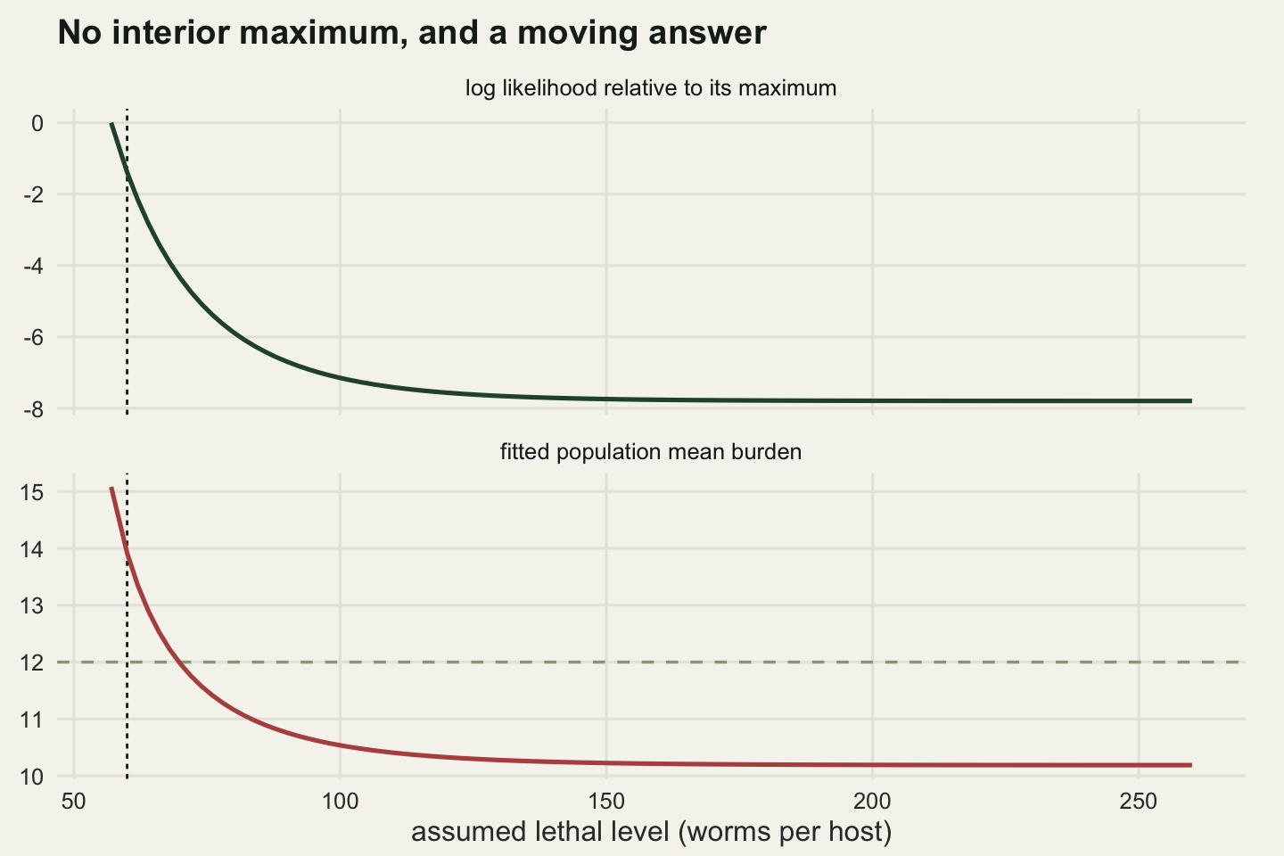
13.9165 10.3259 4.8947 The profile has no interior maximum. It is monotone decreasing in the assumed lethal level, so the likelihood always prefers the smallest cut compatible with the data, which is one more than the largest burden observed. That is not an estimate of a biological quantity. It is a statement about how many hosts were dissected: trap more mice, see a bigger maximum, and the “estimate” moves up. Anderson and Gordon (1982) made the same point about trying to read the mortality out of the shape of the observed distribution.
The size of the effect is the second half of it. Across assumed lethal levels from 57 to 260 worms, the whole log likelihood moves by 7.79 while the estimated population mean moves by 4.89 worms per host. Assuming the true value of 60 gives 13.917; assuming 120 gives 10.326, a drop of 25.8 per cent for a change in an input nobody measured. In the five hundred replicates above, assuming a lethal level of ninety when the truth was sixty gave a mean of 9.841, which is 17.99 per cent short of the truth: about 2.09 standard deviations of an estimator whose standard deviation is 1.035.
The last row of the recovery table is the honest case. Under the smooth survival curve there is no lethal level at all, and applying the right-truncated fit with the cut set to sixty returns a mean of 9.164, still 23.63 per cent short. The correction removed part of the bias and left the rest, and nothing in its output distinguishes that from success.
A second aggregated family, a different missing tail
The right-truncated fit recovers the population mean because the negative binomial carries the missing tail. The data below the cut pin down \(\mu\) and \(k\), and the assumed family then supplies everything above it. Nothing else could: there are no observations up there. The question is how much of the answer that assumption is doing, and the way to find out is to put a different but comparably plausible aggregated family through the same machinery.
The Poisson-lognormal is the natural competitor. Each host has a latent expected burden drawn from a lognormal, and the realised count is Poisson around it. Bulmer (1974) worked out how to fit it, and Shaw, Grenfell and Dobson (1998) found it competitive with the negative binomial across wildlife datasets. It has two parameters like the negative binomial, it produces the same kind of long-tailed aggregated shape, and it has no closed form, so the probability of a count has to be integrated over the latent variable.
Writing the latent variable as \(\log\lambda = m + s Z\) with \(Z\) standard normal turns the probability of a count into an expectation over \(Z\), and the obvious tool is Gauss-Hermite quadrature. Its nodes and weights come from the eigen-decomposition of the Jacobi matrix of the Hermite polynomials, which is a dozen lines of base R. The alternative is a fine grid in \(Z\) with normal weights, which is cruder and, as the comparison below shows, the one to use here.
gauss_hermite <- function(m) {
  idx <- seq_len(m - 1)
  jac <- matrix(0, m, m)
  jac[cbind(idx, idx + 1)] <- sqrt(idx / 2)
  jac[cbind(idx + 1, idx)] <- sqrt(idx / 2)
  eig <- eigen(jac, symmetric = TRUE)
  ord <- order(eig$values)
  list(node = sqrt(2) * eig$values[ord],
       weight = (eig$vectors[1, ord])^2)
}

gh <- gauss_hermite(120)
z_grid <- seq(-8, 8, length.out = 2001)
z_wt <- dnorm(z_grid) * (z_grid[2] - z_grid[1])

mix_pmf <- function(xv, lmean, lsd, node, wt) {
  lam <- exp(lmean + lsd * node)
  as.vector(outer(xv, lam, function(a, b) dpois(a, b)) %*% wt)
}
pln_pmf <- function(xv, lmean, lsd) mix_pmf(xv, lmean, lsd, z_grid, z_wt)

probe <- c(0, 5, 20, 50, 100, 200)
by_hermite <- mix_pmf(probe, 1.86, 2.25, gh$node, gh$weight)
by_grid <- pln_pmf(probe, 1.86, 2.25)
by_integrate <- vapply(probe, function(xi)
  integrate(function(z) dpois(xi, exp(1.86 + 2.25 * z)) * dnorm(z),
            -8, 8, rel.tol = 1e-10)$value, numeric(1))
grid_err <- max(abs(by_grid[-6] / by_integrate[-6] - 1))
hermite_err <- max(abs(by_hermite[-6] / by_integrate[-6] - 1))
print(signif(rbind(count = probe, gauss_hermite_120 = by_hermite,
                   fine_grid = by_grid, adaptive_integrate = by_integrate), 4))
[,1] [,2] [,3] [,4] [,5] [,6]
count 0.000 5.00000 20.000000 50.000000 1.000e+02 2.000e+02
gauss_hermite_120 0.172 0.03426 0.007656 0.001372 5.684e-04 2.891e-04
fine_grid 0.172 0.03432 0.007818 0.002348 8.450e-04 2.765e-04
adaptive_integrate 0.172 0.03432 0.007818 0.002348 8.450e-04 1.599e-14print(round(c(grid_weights_sum_to = sum(z_wt), worst_grid_error = grid_err,
worst_hermite_error = hermite_err), 8))grid_weights_sum_to worst_grid_error worst_hermite_error
1.0000000 0.0000000 0.4158891 The fine grid and integrate agree to eight figures everywhere except the last column, where integrate is the one that has failed: its adaptive subdivision misses a peak that has become very narrow. The Gauss-Hermite rule is wrong by up to 41.6 per cent over the counts probed, and no warning is issued. The reason is that the Poisson kernel, seen as a function of \(\log\lambda\), has width about \(1/\sqrt{x}\), so it narrows as the count grows until it falls between the quadrature nodes; a rule with a fixed number of nodes eventually aliases. This is the sort of thing that produces a plausible fitted curve and a wrong answer, so the grid rule is used from here on.
The right-truncated Poisson-lognormal likelihood is then the same construction as before: the log of the probability at each observed count, minus the sample size times the log of the probability of falling below the cut. Evaluating it on the distinct observed counts with their multiplicities is several times faster and identical. Because the lognormal’s tail runs past the end of any grid, every population quantity below uses the closed-form mean exp(lmean + lsd^2 / 2).
rt_pln_nll <- function(par, tab_x, tab_n, cut_at) {
  px <- pln_pmf(tab_x, par[1], exp(par[2]))
  pc <- sum(pln_pmf(0:(cut_at - 1), par[1], exp(par[2])))
  if (any(px <= 0) || pc <= 0) return(1e10)
  -(sum(tab_n * log(px)) - sum(tab_n) * log(pc))
}

fit_rt_pln <- function(x, cut_at) {
  tally <- table(x)
  tab_x <- as.integer(names(tally))
  tab_n <- as.vector(tally)
  opt <- optim(c(log(mean(x) + 0.5), log(1.5)), rt_pln_nll,
               tab_x = tab_x, tab_n = tab_n, cut_at = cut_at,
               control = list(reltol = 1e-12, maxit = 5000))
  lsd <- exp(opt$par[2])
  c(lmean = opt$par[1], lsd = lsd,
    mu = exp(opt$par[1] + lsd^2 / 2), loglik = -opt$value)
}

fit_pln_one <- fit_rt_pln(burden_obs, lethal)
print(round(fit_pln_one, 4))
lmean lsd mu loglik
2.3781 2.8284 588.6816 -737.3321 nb_tail <- 1 - pnbinom(lethal - 1, size = fit_rt_one["k"], mu = fit_rt_one["mu"])
pln_tail <- 1 - sum(pln_pmf(0:(lethal - 1), fit_pln_one["lmean"],
fit_pln_one["lsd"]))
share_above <- function(prob_low, exact_mean) {
1 - sum((0:(lethal - 1)) * prob_low) / exact_mean
}
nb_share <- unname(share_above(dnbinom(0:(lethal - 1), size = fit_rt_one["k"],
mu = fit_rt_one["mu"]), fit_rt_one["mu"]))
pln_share <- unname(share_above(pln_pmf(0:(lethal - 1), fit_pln_one["lmean"],
fit_pln_one["lsd"]), fit_pln_one["mu"]))
aic_gap <- 2 * (unname(fit_rt_one["loglik"]) - unname(fit_pln_one["loglik"]))
print(round(c(aic_advantage_of_nb = aic_gap,
nb_population_mean = unname(fit_rt_one["mu"]),
pln_population_mean = unname(fit_pln_one["mu"]),
true_population_mean = mu_true), 4)) aic_advantage_of_nb nb_population_mean pln_population_mean
1.7955 13.9165 588.6816
true_population_mean
12.0000 print(round(c(nb_prob_above_lethal = nb_tail,
pln_prob_above_lethal = pln_tail,
true_prob_above_lethal = frac_hosts_lost,
nb_share_of_worms_above = nb_share,
pln_share_of_worms_above = pln_share,
true_share_of_worms_above = frac_worms_lost), 4)) nb_prob_above_lethal pln_prob_above_lethal true_prob_above_lethal
0.0475 0.2732 0.0346
nb_share_of_worms_above pln_share_of_worms_above true_share_of_worms_above
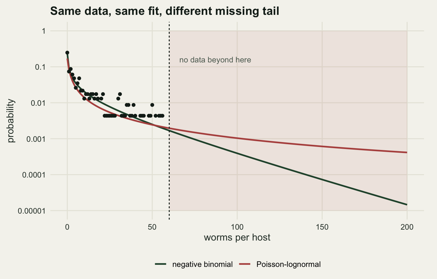
0.3028 0.9871 0.2463 Both models were fitted to the same 230 counts, all of them below 60 worms, with the same number of parameters and the same assumed lethal level. The negative binomial says the population mean is 13.92 worms per host. The Poisson-lognormal says 588.7. The truth is 12, so the negative binomial is right, but only because it is the family the data came from, which is information no field survey has.
The two answers about the missing tail are further apart still. The negative binomial puts 4.75 per cent of hosts above the lethal level and 30.3 per cent of the worms; the Poisson-lognormal puts 27.32 per cent of hosts and 98.7 per cent of the worms there. The true values are 3.46 and 24.6. One model says under a third of the worm population is out of reach; the other says most of it is.
The last thing to check is whether the data can tell them apart. AIC separates the two by 1.8 AIC units. A goodness-of-fit test on the observed range is the fairer question anyway, because a table of observed against expected frequencies is what a field worker would actually inspect.
bin_edges <- c(0, 1, 2, 3, 5, 8, 12, 18, 26, 38, lethal)
observed <- as.vector(table(cut(burden_obs, breaks = bin_edges,
                                right = FALSE, labels = FALSE)))

expected_from <- function(prob_vec) {
  prob_vec <- prob_vec / sum(prob_vec)
  vapply(seq_len(length(bin_edges) - 1), function(i)
    sum(prob_vec[(bin_edges[i] + 1):bin_edges[i + 1]]), numeric(1)) *
    length(burden_obs)
}
exp_nb <- expected_from(dnbinom(0:(lethal - 1), size = fit_rt_one["k"],
                                mu = fit_rt_one["mu"]))
exp_pln <- expected_from(pln_pmf(0:(lethal - 1), fit_pln_one["lmean"],
                                 fit_pln_one["lsd"]))

chisq_of <- function(ex) {
  stat <- sum((observed - ex)^2 / ex)
  dfree <- length(observed) - 1 - 2
  c(statistic = stat, df = dfree, p = pchisq(stat, dfree, lower.tail = FALSE))
}
print(rbind(bin_start = bin_edges[-length(bin_edges)],
            observed = observed, expected_nb = round(exp_nb, 2),
            expected_pln = round(exp_pln, 2)))
[,1] [,2] [,3] [,4] [,5] [,6] [,7] [,8] [,9] [,10]
bin_start 0.00 1.00 2.00 3.00 5.00 8.00 12.00 18.00 26.00 38.00
observed 57.00 17.00 20.00 25.00 25.00 17.00 22.00 14.00 18.00 15.00
expected_nb 56.69 22.42 15.32 21.83 22.46 20.75 21.10 18.26 16.49 14.68
expected_pln 53.78 26.39 17.29 22.99 21.79 18.86 18.56 16.31 16.05 17.98print(round(rbind(negative_binomial = chisq_of(exp_nb),
poisson_lognormal = chisq_of(exp_pln)), 4)) statistic df p
negative_binomial 5.3417 7 0.6183
poisson_lognormal 6.4878 7 0.4841On this survey the negative binomial gives a chi-square p value of 0.618 and the Poisson-lognormal 0.484. Two families fitted to the same visible counts disagree by a factor of 42 about the quantity the survey was run to estimate.
Within the Poisson-lognormal alone the position is no better. Profiling the likelihood over the spread of the latent distribution and reading off the implied population mean shows how little the observed range constrains it.
lsd_seq <- seq(1.6, 4.6, by = 0.05)
pln_tally <- table(burden_obs)
pln_prof <- t(vapply(lsd_seq, function(s_try) {
  opt <- optimize(function(m_try)
    rt_pln_nll(c(m_try, log(s_try)), as.integer(names(pln_tally)),
               as.vector(pln_tally), lethal), c(-2, 7))
  c(lsd = s_try, lmean = opt$minimum, loglik = -opt$objective,
    pop_mean = exp(opt$minimum + s_try^2 / 2))
}, numeric(4)))
pln_prof <- as.data.frame(pln_prof)
pln_prof$delta <- pln_prof$loglik - max(pln_prof$loglik)

within2 <- pln_prof[pln_prof$delta > -2, ]
print(round(pln_prof[seq(1, nrow(pln_prof), by = 6), ], 4))
lsd lmean loglik pop_mean delta
1 1.6 1.5274 -747.8643 16.5663 -10.5312
7 1.9 1.6219 -741.5522 30.7800 -4.2191
13 2.2 1.7922 -738.7479 67.5023 -1.4148
19 2.5 2.0344 -737.6250 174.0532 -0.2920
25 2.8 2.3452 -737.3338 525.9587 -0.0008
31 3.1 2.7221 -737.4565 1857.7338 -0.1234
37 3.4 3.1629 -737.7795 7652.9875 -0.4465
43 3.7 3.6657 -738.1910 36705.2959 -0.8580
49 4.0 4.2291 -738.6314 204662.5805 -1.2984
55 4.3 4.8519 -739.0694 1325031.5939 -1.7364
61 4.6 5.5331 -739.4890 9950316.8839 -2.1560print(c(support_lsd_low = min(within2$lsd), support_lsd_high = max(within2$lsd),
support_mean_low = round(min(within2$pop_mean), 1),
support_mean_high = formatC(max(within2$pop_mean),
format = "e", digits = 2))) support_lsd_low support_lsd_high support_mean_low support_mean_high
"2.15" "4.45" "58.6" "3.56e+06" Every Poisson-lognormal in that set is within two log-likelihood units of the best one, which is the conventional boundary for “the data do not distinguish these”. Across the set the implied population mean runs from 58.6 worms per host to 3.56e+06. The observed counts, all of them below 60, place essentially no upper bound on the burden of the hosts that are not there.
What the field can supply and the likelihood cannot
Two field measures put real information where the likelihood has none, and it is worth knowing what each is worth.
The first is to stop treating the mortality as a cliff. If an experimental infection has calibrated the survival curve, so that the probability of a host with burden \(x\) being alive at trapping time is a known function \(S(x)\), then the survivors follow the survival-weighted distribution \(f(x)S(x)\) divided by its sum, and that is a likelihood like any other. It has no cut in it, which is the point: nothing about it pretends there is a burden above which hosts vanish.
mu_ceiling <- 400

fit_weighted <- function(x, x50_assumed, s_assumed) {
  w_grid <- 1 / (1 + exp((x_grid - x50_assumed) / s_assumed))
  w_obs <- 1 / (1 + exp((x - x50_assumed) / s_assumed))
  opt <- optim(c(log(mean(x) + 0.5), 0), function(par) {
    mu <- exp(par[1])
    kk <- exp(par[2])
    den <- sum(dnbinom(x_grid, size = kk, mu = mu) * w_grid)
    -(nb_loglik(x, mu, kk) + sum(log(w_obs)) - length(x) * log(den))
  }, method = "L-BFGS-B", lower = c(log(0.5), log(0.02)),
  upper = c(log(mu_ceiling), log(50)))
  c(mu = exp(opt$par[1]), k = exp(opt$par[2]))
}

n_rep_w <- 200
set.seed(5150)
w_out <- vapply(seq_len(n_rep_w), function(b) {
  x <- rnbinom(n_host, size = k_true, mu = mu_true)
  soft <- x[runif(n_host) < host_survival(x)]
  c(right = fit_weighted(soft, x50, s_mort),
    gentle = fit_weighted(soft, 1.4 * x50, s_mort),
    harsh = fit_weighted(soft, 0.7 * x50, s_mort))
}, numeric(6))
w_out <- as.data.frame(t(w_out))

w_row <- function(v) c(median = median(v), mean = mean(v), sd = sd(v),
                       ceiling_pct = 100 * mean(v > 0.99 * mu_ceiling))
print(round(rbind(calibration_correct = w_row(w_out$right.mu),
                  half_point_40pct_high = w_row(w_out$gentle.mu),
                  half_point_30pct_low = w_row(w_out$harsh.mu)), 3))
median mean sd ceiling_pct
calibration_correct 12.213 12.459 2.696 0.0
half_point_40pct_high 9.317 9.300 1.202 0.0
half_point_30pct_low 22.082 32.268 49.305 1.5With the survival curve known the weighted fit recovers a mean of 12.459 against a truth of 12, on data where the naive fit returned 7.96. Get the half-survival point wrong in the forgiving direction, forty per cent too high, and it returns 9.3, which is 22.5 per cent short.
The other direction is worse than wrong, it is unbounded. With the half-survival point thirty per cent too low the median estimate is 22.08, nearly double the truth, and in 1.5 per cent of replicates the estimate walks to the ceiling of 400 worms that the optimiser was given. That is not a convergence failure. Assuming mortality is harsher than it is means claiming the observed hosts are improbable survivors, and the model’s only way of explaining them is to push the underlying mean up. Where it stops is set by the analyst’s bounds rather than by the data.
The second measure is to go and collect the missing observations. Carcasses are hard to find and biased in their own ways, but even a few of them turn the problem from extrapolation into interpolation. The likelihood is two pieces sharing one pair of parameters: the trapped hosts are right-truncated at the lethal level, the carcasses are left-truncated at it, and no assumption is needed about their relative sampling rates.
two_piece_fit <- function(alive, dead, cut_at) {
  opt <- optim(c(log(mean(c(alive, dead)) + 0.5), 0), function(par) {
    mu <- exp(par[1])
    kk <- exp(par[2])
    lo <- pnbinom(cut_at - 1, size = kk, mu = mu, log.p = TRUE)
    hi <- pnbinom(cut_at - 1, size = kk, mu = mu, log.p = TRUE,
                  lower.tail = FALSE)
    ll <- nb_loglik(alive, mu, kk) - length(alive) * lo
    if (length(dead)) ll <- ll + nb_loglik(dead, mu, kk) - length(dead) * hi
    -ll
  }, control = list(reltol = 1e-12, maxit = 5000))
  c(mu = exp(opt$par[1]), k = exp(opt$par[2]))
}

draw_carcasses <- function(m) {
  found <- numeric(0)
  while (length(found) < m) {
    pool <- rnbinom(500, size = k_true, mu = mu_true)
    found <- c(found, pool[pool >= lethal])
  }
  found[seq_len(m)]
}

n_rep_c <- 400
carcass_design <- list(c(n_host, 0), c(n_host, 10), c(n_host, 25),
                       c(n_host, 60), c(2 * n_host, 0))
carcass_tab <- t(vapply(carcass_design, function(des) {
  set.seed(31337)
  vals <- vapply(seq_len(n_rep_c), function(b) {
    x <- rnbinom(des[1], size = k_true, mu = mu_true)
    two_piece_fit(x[x < lethal],
                  if (des[2] > 0) draw_carcasses(des[2]) else numeric(0), lethal)
  }, numeric(2))
  c(hosts = des[1], carcasses = des[2], mean_mu = mean(vals[1, ]),
    sd_mu = sd(vals[1, ]), mean_k = mean(vals[2, ]))
}, numeric(5)))
print(round(carcass_tab, 4))
hosts carcasses mean_mu sd_mu mean_k
[1,] 240 0 12.3101 2.6346 0.4039
[2,] 240 10 12.1672 1.8998 0.4061
[3,] 240 25 12.1764 1.6777 0.4013
[4,] 240 60 12.0663 1.2989 0.4027
[5,] 480 0 12.1085 1.6008 0.4046print(round(c(sd_drop_10_carcasses =
100 * (1 - carcass_tab[2, "sd_mu"] / carcass_tab[1, "sd_mu"]),
sd_drop_60_carcasses =
100 * (1 - carcass_tab[4, "sd_mu"] / carcass_tab[1, "sd_mu"]),
sd_drop_doubling_the_survey =
100 * (1 - carcass_tab[5, "sd_mu"] / carcass_tab[1, "sd_mu"])), 3)) sd_drop_10_carcasses.sd_mu sd_drop_60_carcasses.sd_mu
27.890 50.699
sd_drop_doubling_the_survey.sd_mu
39.237 Ten carcasses added to 240 trapped hosts cut the standard deviation of the estimated mean from 2.635 to 1.9, a drop of 27.89 per cent. Sixty carcasses take it to 1.299. The last row is the comparison worth having: doubling the number of hosts dissected, from 240 to 480, buys 39.24 per cent, so twenty-five carcasses were worth about as much as another 240 dissections, and cost a great deal less. They are also the only observations in the study that carry any information at all about the region the estimate depends on.
The honest limit
The estimand here is a property of animals that are not in the population being sampled. The mean burden of the whole host population, including the mice that died of their worms, is not a quantity the survey has partial information about and could get at with a better model. The survey has no information about it. Everything above the lethal level in every fit in this post came out of an assumed distributional family, not out of a measurement.
That is why the right-truncated fit works so well in the recovery section and means so little on its own. It recovered the mean to 12.427 because the data were generated from a negative binomial and it was told they were, and because it was handed the lethal level. Take either away and it moves: the wrong lethal level gave 9.841, and the Poisson-lognormal, told the right lethal level and fitted to the same observed counts, gave 588.7. The spread across assumptions is far larger than the sampling standard deviation of 2.685 that any of those fits would report.
So the correct use of these estimators is a sensitivity analysis, not a recovery. Fit the right-truncated model over the range of lethal levels the biology allows, fit it under two or three aggregated families, and report the envelope. If the envelope is narrow the conclusion is safe; if it spans a factor of 42 between two families, and runs from 58.6 to 3.56e+06 within one of them, as it does here, then the honest report is that the population mean burden was not estimated. Lester (1984) reached the same conclusion by a different route forty years ago, listing methods that are indicative rather than conclusive and saying so in the title of each section.
Three things follow for a field programme. Sample carcasses as well as live hosts, even badly and in small numbers, because twenty-five of them bought as much precision as doubling the trapping effort. Calibrate the survival curve with an experimental infection if the system allows one, and err on the forgiving side, because assuming mortality is harsher than it is sends the estimate to whatever ceiling the optimiser was given rather than to a wrong but finite number. And if neither is possible, report the estimate for what it is: the mean burden of hosts alive at the time of sampling, which the ordinary fit estimates without bias, and which is not the population burden distribution.
A closing note on what did not break. The qualitative statement that burdens are aggregated survived everything done to it here: the Poisson was rejected in 100 per cent of truncated replicates, the top-fifth share fell by 5.25 per cent, and the maximum likelihood \(k\) rose by 11.42 per cent. A paper whose claim is “this parasite is strongly aggregated” is not in trouble. A paper whose claim involves the mean burden, the total parasite population, the variance, or a moment-based aggregation index is in trouble by amounts between 22 and 44 per cent, and nothing in its output says so.
Where to go next
The mechanism has a name outside parasitology. Conditioning on survival is conditioning on a collider, and collider bias and selection works through the same structure where the outcome is a correlation rather than a distribution parameter. The counterpart failure at the other end of the distribution, where the sample has too many zeros rather than too few large values, is in zero-inflated and hurdle models; reading the two together is the quickest way to see that a dispersion statistic on its own cannot say which end of the distribution has been tampered with.
If the survey has covariates, so that the question is how burden varies with host age, sex or site rather than what the marginal distribution looks like, the right-truncated likelihood above extends by replacing \(\mu\) with \(\exp(X\beta)\) and letting each host have its own truncation probability. The regression version of the untruncated fit is in Poisson and negative binomial GLMs in R. Everything in this post about the lethal level being unidentified carries over unchanged, and the extra parameters make it worse rather than better.
References
Crofton HD 1971 Parasitology 62(2):179-193 (10.1017/S0031182000071420)
Crofton HD 1971 Parasitology 63(3):343-364 (10.1017/S0031182000079890)
Bulmer MG 1974 Biometrics 30(1):101-110 (10.2307/2529621)
Anderson RM, Gordon DM 1982 Parasitology 85(2):373-398 (10.1017/S0031182000055347)
Lester RJG 1984 Helgolander Meeresuntersuchungen 37(1):53-64 (10.1007/BF01989295)
Shaw DJ, Dobson AP 1995 Parasitology 111(S1):S111-S133 (10.1017/S0031182000075855)
Wilson K, Grenfell BT, Shaw DJ 1996 Functional Ecology 10(5):592-601 (10.2307/2390169)
Woolhouse MEJ, Dye C, Etard JF, Smith T, Charlwood JD, Garnett GP, Hagan P, Hii JLK, Ndhlovu PD, Quinnell RJ, Watts CH, Chandiwana SK, Anderson RM 1997 Proceedings of the National Academy of Sciences 94(1):338-342 (10.1073/pnas.94.1.338)
Shaw DJ, Grenfell BT, Dobson AP 1998 Parasitology 117(6):597-610 (10.1017/S0031182098003448)