library(ggplot2)

te_paper  <- "#f5f4ee"
te_ink    <- "#16241d"
te_body   <- "#2c3a31"
te_forest <- "#275139"
te_rust   <- "#b5534e"
te_gold   <- "#c9b458"
te_line   <- "#dad9ca"

theme_datasheet <- function() {
  theme_minimal(base_size = 12) +
    theme(plot.background  = element_rect(fill = te_paper, colour = NA),
          panel.background = element_rect(fill = te_paper, colour = NA),
          panel.grid.major = element_line(colour = te_line, linewidth = 0.3),
          panel.grid.minor = element_blank(),
          text             = element_text(colour = te_body),
          plot.title       = element_text(colour = te_ink, face = "bold"),
          plot.subtitle    = element_text(colour = te_body),
          axis.text        = element_text(colour = te_body),
          strip.text       = element_text(colour = te_ink))
}Faecal egg count reduction tests at low counts
R
parasitology
disease ecology
bootstrap
simulation
ecology tutorial
At McMaster egg counts a drug that works 99 per cent usually reads as 100 and its interval collapses. Coverage and resistance calls are measured in R.
A smallholder with ten ewes wants to know whether the white drench still works. The vet takes a faecal sample from each ewe on the day of treatment and again two weeks later, and the laboratory counts eggs on a McMaster slide. One egg seen under the grid is recorded as fifty eggs per gram of faeces, because the chamber holds a fixed fraction of a diluted sample. The pre-treatment counts come back at a few hundred eggs per gram, the post-treatment counts are all zero, and the report says the drug reduced egg output by 100 per cent. A bootstrap interval, if anyone computes one, runs from 100 to 100.
The faecal egg count reduction test is the standard field test for anthelmintic resistance in sheep, goats, cattle and horses. In its paired form it divides the mean post-treatment count by the mean pre-treatment count and compares the reduction with a threshold. The problem this post measures is well known in veterinary parasitology, and nothing here is a new result. Levecke and colleagues (2012) showed by simulation that the outcome of the test depends on the detection limit of the counting method, the number of animals and the level and aggregation of egg output; Torgerson, Paul and Furrer (2014) built the eggCounts package around a model that treats the slide count, not the eggs per gram, as the observation; and the 2023 guideline of the World Association for the Advancement of Veterinary Parasitology (Kaplan and colleagues 2023) replaced the 1992 rule (Coles and colleagues 1992) with one that sizes the test by the number of eggs counted and asks for positive evidence before calling a drug either susceptible or resistant. What the post adds is a small, runnable demonstration: how often the report reads 100, how often its interval covers the truth, and how often a resistant drug is called, under both rules.
Three posts on this site deal with measurements that stop resolving at the low end, and none of them is this problem. Values below the detection limit treats a continuous concentration that is censored below a limit and fits the censored likelihood; its test is a trend regression, and nothing in it is a ratio or a treatment decision. Rounded and coarsened measurements works with a known grid that adds a fixed amount of variance to a continuous value. Parasite burdens truncated by host death is about worm counts and the aggregation parameter. Here the limit is a counting multiplier applied to aggregated counts, and it acts on a ratio at its top end, which is exactly where the treatment decision sits. The failure of the bootstrap that follows is a cousin of the one in checking a bootstrap, where resampling cannot produce a value beyond the sample maximum: here it cannot produce a post-treatment egg when none was counted.
The generating model and three intervals
Each animal carries its own true egg output, drawn from a gamma distribution with mean 150 eggs per gram and shape 0.7, so that egg output is strongly aggregated: a few animals carry most of the eggs. Egg output also varies from day to day within an animal, with a coefficient of variation of 0.3, drawn independently for the two sampling days. The treatment multiplies the animal’s output by one minus the efficacy. The slide sees a Poisson number of eggs with mean equal to the output divided by the multiplication factor, and the laboratory reports that count times the factor. All of these constants were fixed before anything was run.
cv_day   <- 0.3                 # day-to-day excretion CV within an animal
shp_day  <- 1 / cv_day^2
k_set    <- 0.7                 # gamma shape of egg output among animals
mu_set   <- 150                 # mean eggs per gram before treatment
n_set    <- 10                  # animals in the treatment group
mf_set   <- 50                  # McMaster multiplication factor
eff_set  <- 0.99                # true efficacy
n_rep    <- 600                 # simulated tests per design cell
n_boot   <- 999                 # paired bootstrap resamples per test
mcse_max <- sqrt(0.25 / n_rep)

sim_test <- function(R, n, mu, k, mf, eff) {
  epg  <- matrix(rgamma(R * n, shape = k, rate = k / mu), R)
  pre  <- matrix(rpois(R * n, epg * rgamma(R * n, shp_day, shp_day) / mf), R)
  post <- matrix(rpois(R * n, epg * (1 - eff) * rgamma(R * n, shp_day, shp_day) / mf), R)
  list(pre = pre, post = post, mf = mf)   # raw eggs seen on the slide
}

fecr_of <- function(tst) 100 * (1 - rowSums(tst$post) / rowSums(tst$pre))
The reduction is computed from group arithmetic means, as in the 1992 guideline; the 2023 guideline moves the decision onto the interval instead of a prescribed mean. The multiplication factor cancels from that ratio, so the point estimate can be computed from raw slide counts. The intervals are where the choices differ, and three are compared.
The first is a paired bootstrap: resample animals with replacement, keeping each animal’s two counts together, and take percentiles of the resampled reduction. Resampling animals is the same as drawing multinomial weights for them, which lets all resamples of all simulated tests be computed with two matrix products.
boot_lim <- function(tst, probs, B = n_boot) {
  n_an  <- ncol(tst$pre)
  wts   <- rmultinom(B, n_an, rep(1 / n_an, n_an))
  bpre  <- tst$pre %*% wts
  bpost <- tst$post %*% wts
  bf <- 100 * (1 - bpost / bpre)
  bf[!is.finite(bf)] <- NA          # resamples with no pre-treatment eggs
  t(apply(bf, 1, quantile, probs = probs, na.rm = TRUE, names = FALSE))
}
The second uses the counts. Under the model in the eggCounts package, an animal’s pre- and post-treatment slide counts are Poisson with means proportional to the same gamma-distributed output, the second multiplied by one minus the efficacy. Conditional on the animal’s total count, its post-treatment count is then binomial with probability r over one plus r, where r is one minus the efficacy, and the animal’s own output drops out. The profile likelihood for the efficacy is therefore a binomial likelihood in the share of all counted eggs that were counted after treatment, whatever the aggregation. The interval below inverts that likelihood ratio. When no post-treatment egg is seen its lower limit has a closed form that depends only on the number of eggs counted, which is the quantity the bootstrap never sees.
The day-to-day variation breaks the binomial step, because the two days no longer share one mean. The third interval is the quasi-likelihood version of the second: it estimates a dispersion from the Pearson residuals across animals, divides the likelihood ratio by it when it exceeds one, and uses an F critical value.
to_eff <- function(p_share) 100 * (1 - p_share / (1 - p_share))

lik_lim <- function(tst, level, quasi = FALSE) {
  z_post <- rowSums(tst$post)
  n_all  <- rowSums(tst$pre) + z_post
  p_hat  <- z_post / n_all
  loglik <- function(p) ifelse(z_post > 0, z_post * log(p), 0) +
    ifelse(n_all - z_post > 0, (n_all - z_post) * log1p(-p), 0)
  l_max <- loglik(p_hat)
  phi  <- rep(1, length(z_post))
  crit <- rep(qchisq(level, 1), length(z_post))
  if (quasi) {
    tot_an <- tst$pre + tst$post
    pear <- ifelse(tot_an > 0, (tst$post - tot_an * p_hat)^2 /
                     (tot_an * p_hat * (1 - p_hat)), 0)
    df_an <- pmax(rowSums(tot_an > 0) - 1, 1)
    phi_raw <- rowSums(pear) / df_an
    over <- z_post > 0 & z_post < n_all & phi_raw > 1
    phi[over]  <- phi_raw[over]
    crit[over] <- qf(level, 1, df_an[over])
  }
  gap <- function(p) 2 * (l_max - loglik(p)) / phi - crit
  bisect <- function(lo, hi, upper_side) {
    for (it in 1:60) {
      mid <- (lo + hi) / 2
      inside <- gap(mid) < 0
      if (upper_side) {
        lo <- ifelse(inside, mid, lo); hi <- ifelse(inside, hi, mid)
      } else {
        hi <- ifelse(inside, mid, hi); lo <- ifelse(inside, lo, mid)
      }
    }
    (lo + hi) / 2
  }
  p_up <- bisect(p_hat, rep(1 - 1e-12, length(p_hat)), TRUE)
  p_lo <- ifelse(z_post == 0, 0, bisect(rep(1e-300, length(p_hat)), p_hat, FALSE))
  cbind(lo = to_eff(p_up), hi = to_eff(p_lo))
}
Ten ewes and a factor of fifty
set.seed(4417)
ex_draws <- sim_test(20, n_set, mu_set, k_set, mf_set, eff_set)
all_zero <- which(rowSums(ex_draws$post) == 0 & rowSums(ex_draws$pre) > 0)
i_ex <- all_zero[1]
ex <- list(pre  = ex_draws$pre[i_ex, , drop = FALSE],
           post = ex_draws$post[i_ex, , drop = FALSE], mf = mf_set)
ex_epg_pre  <- mf_set * ex$pre
ex_mean_pre <- mean(ex_epg_pre)
ex_eggs     <- sum(ex$pre)
ex_zero_pre <- sum(ex$pre == 0)
ex_max_epg  <- max(ex_epg_pre)
ex_fecr     <- fecr_of(ex)
ex_boot     <- boot_lim(ex, c(0.025, 0.975))
ex_lik      <- lik_lim(ex, 0.95)
ex_lo_closed <- to_eff(1 - exp(-qchisq(0.95, 1) / (2 * ex_eggs)))
ex_epg_pre
[,1] [,2] [,3] [,4] [,5] [,6] [,7] [,8] [,9] [,10]
[1,] 100 50 250 450 100 50 0 150 0 50This is the first of twenty simulated tests from the design above in which no egg was seen after treatment, and it was taken as the first such draw rather than chosen. The ten ewes had a mean pre-treatment count of 120 eggs per gram, the largest 450, and 2 of them showed no egg at all before treatment. Behind that mean are 24 eggs actually counted under the microscope. The reported reduction is 100 per cent against a true 99.
The paired bootstrap interval runs from 100.0 to 100.0. Every resample contains only zeros after treatment, so every resampled reduction is 100, and the interval has no width at all. The likelihood interval runs from 91.7 to 100.0. Its lower limit has a closed form. With no post-treatment egg among 24 counted, the likelihood ratio reaches the chi-squared critical value at a post-treatment share of one minus the exponential of minus 1.92 over 24, which is an efficacy of 91.7, and the interval says what the slide supports: a drug somewhere above about nine tenths effective, with no evidence either way about 95 or 99 per cent.
How often a 99 per cent drug reads as 100
The report of exactly 100 per cent happens when every post-treatment slide is empty, and that probability has a closed form. If every animal excreted the same number of eggs per gram, the post-treatment total would be Poisson with mean n times the output times one minus the efficacy, divided by the factor, and the chance of seeing nothing is the exponential of minus that. With gamma-distributed output among animals each slide is empty with the negative binomial zero probability, and the group probability is its n-th power. The day-to-day variation is not in either formula, so the simulation checks how much it matters.
mf_grid  <- c(50, 25, 15, 1)
n_grid   <- c(10, 20, 40)
eff_grid <- c(0.99, 0.95, 0.90)
n_zero_rep <- 20000

p_zero_fixed <- function(n, mu, mf, eff) exp(-n * mu * (1 - eff) / mf)
p_zero_gamma <- function(n, mu, k, mf, eff) (1 + mu * (1 - eff) / (k * mf))^(-k * n)
pz_fixed_set <- p_zero_fixed(n_set, mu_set, mf_set, eff_set)
pz_gamma_set <- p_zero_gamma(n_set, mu_set, k_set, mf_set, eff_set)

set.seed(2023)
zero_tab <- do.call(rbind, lapply(n_grid, function(n_an) {
  do.call(rbind, lapply(mf_grid, function(mf) {
    tst <- sim_test(n_zero_rep, n_an, mu_set, k_set, mf, eff_set)
    ok  <- rowSums(tst$pre) > 0
    data.frame(n = n_an, mf = mf,
               sim   = mean(rowSums(tst$post)[ok] == 0),
               fixed = p_zero_fixed(n_an, mu_set, mf, eff_set),
               gamma = p_zero_gamma(n_an, mu_set, k_set, mf, eff_set))
  }))
}))
zero_gap_gamma <- max(abs(zero_tab$sim - zero_tab$gamma))
zero_gap_fixed <- max(abs(zero_tab$sim - zero_tab$fixed))
mcse_zero <- sqrt(0.25 / n_zero_rep)
zt <- function(n_an, mf, col) zero_tab[zero_tab$n == n_an & zero_tab$mf == mf, col]
For ten animals at 150 eggs per gram and a factor of 50, the fixed-output formula gives 0.741 and the gamma formula 0.745. Simulating 20000 tests per design gives 0.749. Across all twelve designs the gamma formula stays within 0.0048 of the simulation, against a Monte Carlo standard error of at most 0.0035, so day-to-day variation barely moves this probability; the fixed-output formula is off by up to 0.030, because aggregation concentrates the eggs in fewer animals and leaves more slides empty.
The exponent is the whole story: n times the mean count times one minus the efficacy, over the factor, is the expected number of eggs on all post-treatment slides together. At a factor of 50 that is 0.3 eggs for ten animals. Doubling the animals and switching to a factor of 15 raises it to 2.0, and the share of empty post-treatment totals falls to 0.159. Only the method that counts every egg (factor 1) removes the problem outright.
zero_tab$group <- factor(sprintf("%d animals", zero_tab$n),
                         levels = sprintf("%d animals", n_grid))
mf_fine <- exp(seq(log(1), log(50), length.out = 120))
zero_curve <- do.call(rbind, lapply(n_grid, function(n_an)
  data.frame(mf = mf_fine, gamma = p_zero_gamma(n_an, mu_set, k_set, mf_fine, eff_set),
             group = factor(sprintf("%d animals", n_an), levels = levels(zero_tab$group)))))
ggplot(zero_tab, aes(mf, sim, colour = group)) +
  geom_line(data = zero_curve, aes(y = gamma), linewidth = 0.9) +
  geom_point(size = 2.4) +
  scale_x_log10(breaks = c(1, 2, 5, 15, 25, 50)) +
  scale_colour_manual(values = c(te_rust, te_gold, te_forest), name = NULL) +
  scale_y_continuous(limits = c(0, 1)) +
  labs(x = "multiplication factor (eggs per gram per egg seen)",
       y = "share reporting exactly 100 per cent",
       title = "A perfect result is mostly a counting result",
       subtitle = "true efficacy 99 per cent, mean 150 eggs per gram, shape 0.7") +
  theme_datasheet() + theme(legend.position = "bottom")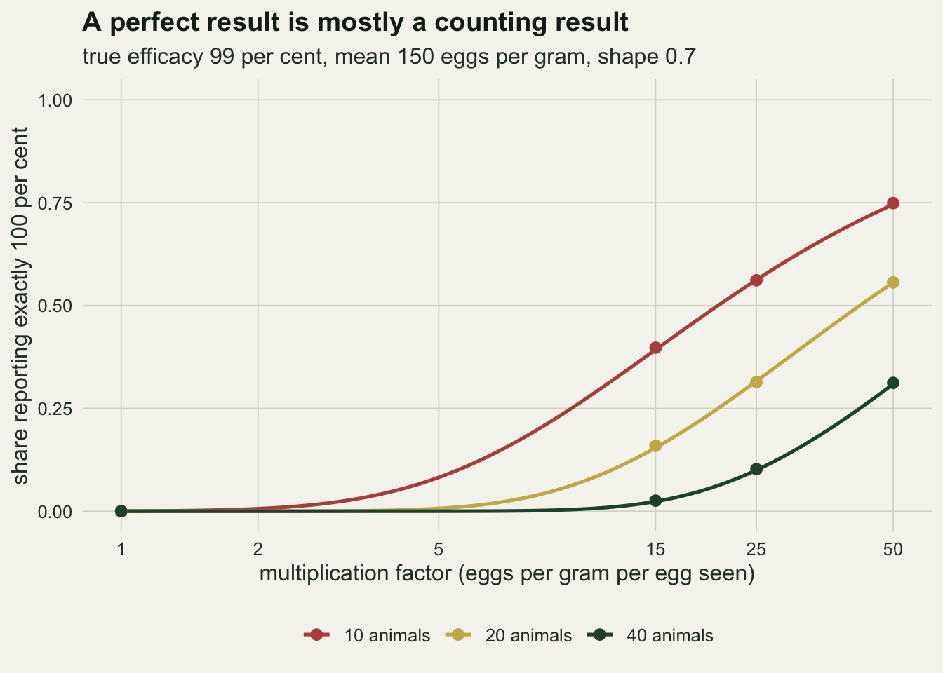
The bootstrap interval collapses where the counts do
The share reporting 100 is arithmetic. The interval is not, so it is measured. Each design cell below simulates 600 tests, a number fixed before running, which puts the Monte Carlo standard error of any coverage at 0.020 or less. Tests with no egg at all before treatment are dropped, as a laboratory would drop them.
run_cell <- function(n, mu, k, mf, eff, R = n_rep) {
  tst <- sim_test(R, n, mu, k, mf, eff)
  ok  <- rowSums(tst$pre) > 0
  tst$pre  <- tst$pre[ok, , drop = FALSE]
  tst$post <- tst$post[ok, , drop = FALSE]
  fecr <- fecr_of(tst)
  bq  <- boot_lim(tst, c(0.025, 0.05, 0.95, 0.975))
  l95 <- lik_lim(tst, 0.95);               l90 <- lik_lim(tst, 0.90)
  q95 <- lik_lim(tst, 0.95, quasi = TRUE); q90 <- lik_lim(tst, 0.90, quasi = TRUE)
  te <- 100 * eff
  covers  <- function(lo, hi) mean(lo <= te & hi >= te)
  class23 <- function(lo, hi) c(res = mean(hi < 99), sus = mean(lo >= 95 & hi >= 99))
  c23b <- class23(bq[, 2], bq[, 3])
  c23l <- class23(l90[, 1], l90[, 2])
  c23q <- class23(q90[, 1], q90[, 2])
  data.frame(n = n, mu = mu, k = k, mf = mf, eff = eff, used = sum(ok),
             eggs = n * mu / mf, rep100 = mean(fecr == 100),
             cov_boot = covers(bq[, 1], bq[, 4]), cov_lik = covers(l95[, 1], l95[, 2]),
             cov_quasi = covers(q95[, 1], q95[, 2]),
             r92_boot = mean(fecr < 95 & bq[, 1] < 90),
             r92_lik  = mean(fecr < 95 & l95[, 1] < 90),
             res_boot = c23b[["res"]], sus_boot = c23b[["sus"]],
             res_lik = c23l[["res"]], sus_lik = c23l[["sus"]],
             res_quasi = c23q[["res"]], sus_quasi = c23q[["sus"]])
}

set.seed(1992)
grid_tab <- do.call(rbind, lapply(eff_grid, function(e) do.call(rbind,
  lapply(n_grid, function(n_an) do.call(rbind,
    lapply(mf_grid, function(mf) run_cell(n_an, mu_set, k_set, mf, e)))))))

gv <- function(n_an, mf, e, col) grid_tab[grid_tab$n == n_an & grid_tab$mf == mf &
                                             abs(grid_tab$eff - e) < 1e-9, col]
n_dropped <- sum(n_rep - grid_tab$used)
top <- grid_tab[abs(grid_tab$eff - 0.99) < 1e-9, ]
boot_low_eggs <- range(top$cov_boot[top$eggs <= 60])
lik_mf1  <- range(grid_tab$cov_lik[grid_tab$mf == 1])
quasi_all <- range(grid_tab$cov_quasi)
quasi_mf1 <- range(grid_tab$cov_quasi[grid_tab$mf == 1])
quasi_rest_min <- min(grid_tab$cov_quasi[grid_tab$mf != 1])
boot_90 <- range(grid_tab$cov_boot[abs(grid_tab$eff - 0.90) < 1e-9])
At ten animals and a factor of 50 the 99 per cent drug reports exactly 100 in 0.758 of tests, and the paired bootstrap interval covers the true 99 in 0.242, against a nominal 0.95 (0 of the 21600 simulated tests in the grid were dropped for an empty pre-treatment slide). Where the grid expects 60 or fewer eggs to be counted before treatment, its coverage for this drug is between 0.242 and 0.457. Twenty animals at a factor of 15 lift the coverage to 0.813, and forty animals at a factor of 1 give 0.933.
The likelihood interval, on exactly the same simulated counts, covers the true 99 in 0.982 of tests at ten animals and a factor of 50. It does not need more counting to be honest at the top end, because a count of zero out of a known number of eggs is information it can use. It fails in the opposite corner. When every egg is counted, day-to-day variation in excretion is larger than the Poisson counting noise the binomial assumes, and the plain likelihood interval covers between 0.543 and 0.892 across the factor-of-1 designs, worst for the less effective drugs. The quasi-likelihood interval, which estimates that extra variation from the animals, covers between 0.842 and 0.988 across all thirty-six cells; every cell in which it falls below 0.913 is a factor-of-1 design (those range from 0.842 to 0.948), where a dispersion estimated from ten to forty aggregated animals is itself noisy.
cov_long <- do.call(rbind, lapply(
  list(c("cov_boot", "paired bootstrap"), c("cov_lik", "binomial likelihood"),
       c("cov_quasi", "quasi-likelihood")), function(m)
    data.frame(eggs = grid_tab$eggs, eff = grid_tab$eff, cover = grid_tab[[m[1]]],
               interval = m[2])))
cov_long$interval <- factor(cov_long$interval,
                            levels = c("paired bootstrap", "binomial likelihood", "quasi-likelihood"))
cov_long$panel <- factor(sprintf("true efficacy %.0f per cent", 100 * cov_long$eff),
                         levels = sprintf("true efficacy %.0f per cent", 100 * eff_grid))
cov_mean <- aggregate(cover ~ eggs + panel + interval, data = cov_long, FUN = mean)

ggplot(cov_long, aes(eggs, cover, colour = interval)) +
  geom_hline(yintercept = 0.95, linetype = "dashed", colour = te_body, linewidth = 0.5) +
  geom_line(data = cov_mean, linewidth = 0.8) +
  geom_point(size = 2, alpha = 0.9) +
  facet_wrap(~ panel, ncol = 3) +
  scale_x_log10(breaks = c(30, 100, 300, 1000, 3000)) +
  scale_colour_manual(values = c(te_rust, te_gold, te_forest), name = NULL) +
  scale_y_continuous(limits = c(0, 1)) +
  labs(x = "eggs expected on the pre-treatment slides (log scale)",
       y = "coverage of the true efficacy",
       title = "Each interval fails at a different end",
       subtitle = "dashed line: nominal 0.95; lines join cell means at equal egg totals") +
  theme_datasheet() + theme(legend.position = "bottom", panel.spacing.x = unit(1.2, "lines"))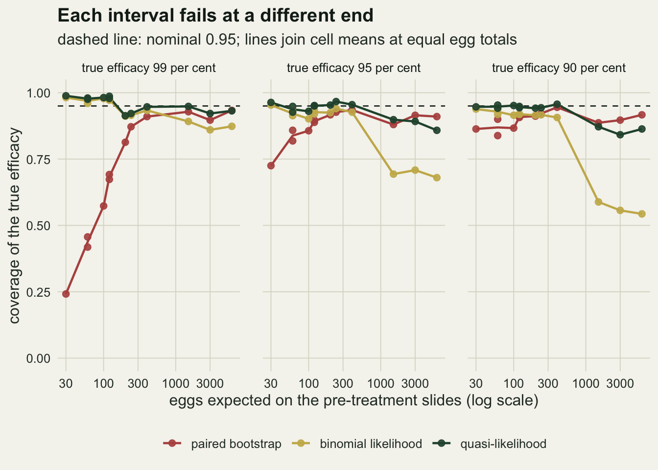
For the effective drug the horizontal axis carries most of the pattern. Ten animals at a factor of 25 and twenty animals at a factor of 50 both expect 60 eggs on the pre-treatment slides, and their bootstrap coverages for the 99 per cent drug are 0.418 and 0.457. For the 90 per cent drug the bootstrap is at or below nominal across the whole grid, between 0.838 and 0.945, but never collapses, because post-treatment eggs are seen in most tests and the resamples have something to vary.
Calling resistance under the 1992 and 2023 rules
The 1992 rule calls resistance when the reduction is below 95 per cent and the lower limit of the 95 per cent interval is below 90. The original rule was written for a treated group against an untreated control, with a variance formula for the interval; here it is applied to the paired design with the bootstrap and likelihood intervals. The 2023 guideline recommends the paired design, uses a 90 per cent interval, and compares it with two numbers for the host and drug: an expected efficacy, 99 per cent in the guideline’s sheep example, and a lower efficacy threshold, taken here as 95 per cent (the research protocol’s grey zone of 95 to 99; the clinical protocol uses 90 to 99). A test is resistant when the upper limit is below the expected efficacy, susceptible when the lower limit reaches the threshold and the upper limit reaches the expected efficacy, and inconclusive otherwise. The guideline suggests a Bayesian approach built for these data and recommends one of two web tools for the analysis (the Bayesian eggCounts interface, or fecrt.com with a hybrid frequentist and Bayesian method) unless a qualified statistician does it, and warns that only a few formulae give an interval when the observed reduction is 100 per cent; the bootstrap below is what a laboratory gets if it ignores that advice, and the likelihood intervals are a frequentist stand-in for the model-based analysis, not the analysis itself. The guideline also sizes the treatment group by the total number of eggs counted before the multiplication factor is applied, not by a minimum count per animal.
c92_boot_10 <- gv(10, 50, 0.90, "r92_boot"); c92_boot_20 <- gv(20, 15, 0.90, "r92_boot")
c92_lik_10  <- gv(10, 50, 0.90, "r92_lik")
fp92_max    <- max(grid_tab$r92_boot[abs(grid_tab$eff - 0.99) < 1e-9])

# the headline cell gets its own, larger run so its rate carries a small MC error
n_rep_esc <- 5000
set.seed(1992 + 10)
esc_tst <- sim_test(n_rep_esc, n_set, mu_set, k_set, mf_set, 0.90)
esc_ok  <- rowSums(esc_tst$pre) > 0
esc_tst$pre <- esc_tst$pre[esc_ok, ]; esc_tst$post <- esc_tst$post[esc_ok, ]
esc_fecr <- fecr_of(esc_tst)
esc_call_boot <- mean(esc_fecr < 95 & boot_lim(esc_tst, c(0.025, 0.975))[, 1] < 90)
esc_call_lik  <- mean(esc_fecr < 95 & lik_lim(esc_tst, 0.95)[, "lo"] < 90)
escape_10   <- 1 - esc_call_boot
mcse_grid_esc <- sqrt(c92_boot_10 * (1 - c92_boot_10) / gv(10, 50, 0.90, "used"))
mcse_escape <- sqrt(escape_10 * (1 - escape_10) / sum(esc_ok))
esc_hi_fecr <- mean(esc_fecr >= 95)

designs <- data.frame(n = c(10, 20, 40), mf = c(50, 15, 1),
                      lab = c("10 animals, factor 50", "20 animals, factor 15",
                              "40 animals, factor 1"))
set.seed(1203)
miss_tst <- sim_test(n_rep, n_set, mu_set, k_set, mf_set, 0.90)
miss_ok  <- rowSums(miss_tst$pre) > 0
miss_tst$pre <- miss_tst$pre[miss_ok, ]; miss_tst$post <- miss_tst$post[miss_ok, ]
miss_up  <- boot_lim(miss_tst, c(0.05, 0.95))[, 2]
missed   <- miss_up >= 99
miss_at100 <- mean(miss_up[missed] == 100)
miss_few   <- mean(rowSums(miss_tst$post[missed, ] > 0) <= 2)

class_long <- do.call(rbind, lapply(seq_len(nrow(designs)), function(i) {
  do.call(rbind, lapply(eff_grid, function(e) {
    do.call(rbind, lapply(list(c("boot", "bootstrap"), c("lik", "likelihood"),
                               c("quasi", "quasi")), function(m) {
      res <- gv(designs$n[i], designs$mf[i], e, paste0("res_", m[1]))
      sus <- gv(designs$n[i], designs$mf[i], e, paste0("sus_", m[1]))
      data.frame(design = designs$lab[i], eff = e, interval = m[2],
                 class = c("resistant", "inconclusive", "susceptible"),
                 share = c(res, 1 - res - sus, sus))
    }))
  }))
}))
With ten animals and a factor of 50, a drug that removes only 90 per cent of egg output is called resistant by the 1992 rule with the bootstrap in 0.805 of the grid’s 600 tests. Because this is the headline cell, it was rerun on its own with 5000 tests: the drug escapes a resistance call in 0.236 of them (Monte Carlo standard error 0.006), a little under one test in four (the grid’s run put the escape at 0.195, a low draw given its own standard error of 0.016). The likelihood interval barely changes this, calling resistance in 0.773 against 0.764 for the bootstrap on the same counts, because the escapes come from the point estimate: the rule needs the reduction itself below 95, and with 30 eggs expected on the pre-treatment slides the 90 per cent drug shows a reduction of 95 or more in 0.227 of tests. Twenty animals at a factor of 15 raise the call rate to 0.937. The 1992 rule never calls a 99 per cent drug resistant in more than 0.060 of tests in this grid.
The 2023 rule fed a bootstrap interval fails at low counts in both directions. For ten animals at a factor of 50, it calls the 99 per cent drug susceptible in 0.793 of tests, on the strength of an interval that has collapsed onto 100, and calls the 90 per cent drug resistant in only 0.385. It even calls a 95 per cent drug, which is below the expected efficacy, susceptible in 0.273. The likelihood interval on the same counts calls the 90 per cent drug resistant in 0.778, the 99 per cent drug susceptible in only 0.377, and the 95 per cent drug susceptible in 0.082; its most common answer for the effective drug is inconclusive, in 0.587 of tests, which is what 30 expected eggs can support.
The missed resistance calls for the 90 per cent drug have a plain cause. In a separate run of 600 such tests, 380 were not called resistant; among those, the share with an upper bootstrap limit of exactly 100 was 1.000, and the share whose post-treatment eggs came from two animals or fewer was 1.000. Resamples that leave those animals out read 100, and there are enough of them to hold the upper limit there.
class_long$class <- factor(class_long$class, levels = c("resistant", "inconclusive", "susceptible"))
class_long$interval <- factor(class_long$interval, levels = c("bootstrap", "likelihood", "quasi"))
class_long$design <- factor(class_long$design, levels = designs$lab)
class_long$effl <- factor(sprintf("true %.0f%%", 100 * class_long$eff),
                          levels = sprintf("true %.0f%%", 100 * eff_grid))
ggplot(class_long, aes(interval, share, fill = class)) +
  geom_col(width = 0.75, colour = te_paper, linewidth = 0.3) +
  facet_grid(effl ~ design) +
  scale_fill_manual(values = c(te_rust, te_line, te_forest), name = NULL) +
  scale_y_continuous(breaks = c(0, 0.5, 1)) +
  labs(x = NULL, y = "share of simulated tests",
       title = "A bootstrap interval misleads the 2023 rule",
       subtitle = "rows: true efficacy; columns: design") +
  theme_datasheet() +
  theme(legend.position = "bottom", axis.text.x = element_text(size = 9))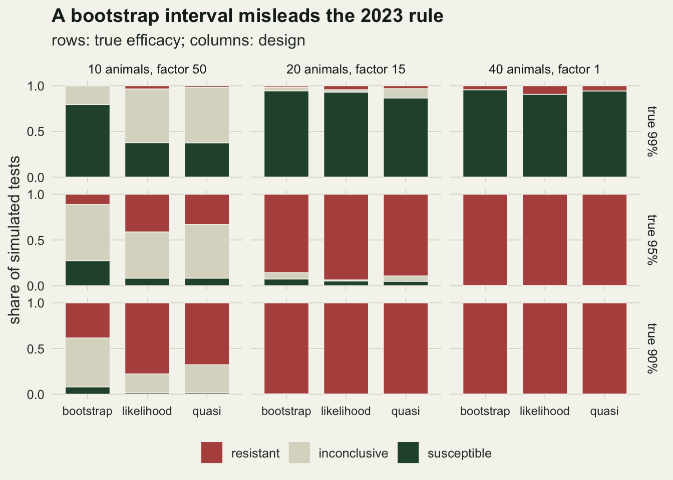
With forty animals counted at a factor of 1 the three intervals agree on the classification almost everywhere. The one visible difference there is that the plain likelihood interval calls the 99 per cent drug resistant in 0.095 of tests against 0.045 for the bootstrap, which is its undercoverage at high counts turning into false alarms.
Aggregation matters less than the eggs counted
The negative binomial shape and the mean count were both held fixed above. The grid below varies them at twenty animals and a factor of 50, for the 99 and 90 per cent drugs.
k_grid  <- c(0.3, 0.7, 2)
mu_grid <- c(50, 150, 600)
set.seed(3009)
agg_tab <- do.call(rbind, lapply(c(0.99, 0.90), function(e) do.call(rbind,
  lapply(k_grid, function(kk) do.call(rbind,
    lapply(mu_grid, function(mu) run_cell(20, mu, kk, mf_set, e)))))))
av <- function(kk, mu, e, col) agg_tab[agg_tab$k == kk & agg_tab$mu == mu &
                                         abs(agg_tab$eff - e) < 1e-9, col]
agg_top <- agg_tab[abs(agg_tab$eff - 0.99) < 1e-9, ]
spread_k_top <- max(tapply(agg_top$cov_boot, agg_top$mu, function(v) diff(range(v))))
spread_mu_top <- max(tapply(agg_top$cov_boot, agg_top$k, function(v) diff(range(v))))
agg_low <- agg_tab[abs(agg_tab$eff - 0.90) < 1e-9, ]
spread_k_low  <- max(tapply(agg_low$cov_boot, agg_low$mu, function(v) diff(range(v))))
spread_mu_low <- max(tapply(agg_low$cov_boot, agg_low$k, function(v) diff(range(v))))
For the 99 per cent drug, changing the shape from 0.3 to 2 at a fixed mean moves the bootstrap coverage by at most 0.118, while changing the mean from 50 to 600 at a fixed shape moves it by up to 0.697. At a mean of 50 eggs per gram, twenty animals expect twenty eggs on their slides, and the bootstrap covers the true 99 in 0.205 of tests at shape 0.7. The likelihood interval covers in 0.982 there.
For the 90 per cent drug the two effects are of similar size, because eggs are seen after treatment and the bootstrap is resampling a skewed ratio rather than a column of zeros: the shape moves its coverage by up to 0.107 and the mean by up to 0.142. At a mean of 50, its coverage is 0.747 at shape 0.3 and 0.853 at shape 2; the quasi-likelihood interval covers 0.942 and 0.943.
agg_long <- rbind(
  data.frame(agg_tab[, c("k", "mu", "eff")], cover = agg_tab$cov_boot, interval = "paired bootstrap"),
  data.frame(agg_tab[, c("k", "mu", "eff")], cover = agg_tab$cov_quasi, interval = "quasi-likelihood"))
agg_long$shape <- factor(sprintf("shape %.1f", agg_long$k), levels = sprintf("shape %.1f", k_grid))
agg_long$panel <- factor(sprintf("true efficacy %.0f per cent", 100 * agg_long$eff),
                         levels = sprintf("true efficacy %.0f per cent", c(99, 90)))
ggplot(agg_long, aes(mu, cover, colour = shape, linetype = interval)) +
  geom_hline(yintercept = 0.95, linetype = "dashed", colour = te_body, linewidth = 0.5) +
  geom_line(linewidth = 0.8) + geom_point(size = 2) +
  facet_wrap(~ panel) +
  scale_x_log10(breaks = mu_grid) +
  scale_colour_manual(values = c(te_rust, te_gold, te_forest), name = NULL) +
  scale_linetype_manual(values = c("solid", "longdash"), name = NULL) +
  scale_y_continuous(limits = c(0, 1)) +
  guides(colour = guide_legend(order = 1), linetype = guide_legend(order = 2, nrow = 2)) +
  labs(x = "mean eggs per gram before treatment (log scale)", y = "coverage of the true efficacy",
       title = "The mean count sets the failure",
       subtitle = "twenty animals, factor 50; dashed line: nominal 0.95") +
  theme_datasheet() + theme(legend.position = "bottom", legend.key.width = unit(2.2, "lines"),
                          panel.spacing.x = unit(2, "lines"))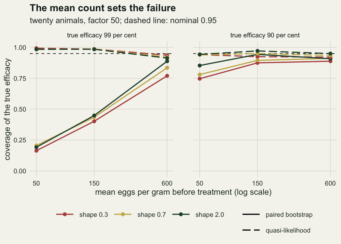
What to report
Report the raw number of eggs counted before and after treatment, as well as the multiplication factor. Those two totals are the information in the test; the eggs per gram figures are a rescaling of them, and a reduction of 100 per cent from 30 eggs means something quite different from 100 per cent from 3000.
Do not report a bootstrap interval of zero width. When every post-treatment count is zero the paired bootstrap has nothing to resample and returns the point estimate twice; quoting it as an interval invites the reader to treat a counting result as a precise one. A likelihood interval on the counts, whose lower limit depends on the eggs counted, is a defensible replacement at low counts, and the model-based Bayesian intervals in eggCounts are built on the same observation; analysing the counts with a method built for these data is also the guideline’s own advice.
Say which rule was applied and with which interval. Under the 2023 rule the interval is the whole decision, and the same counts produced a susceptible call for the effective drug in 0.793 of tests with one interval and 0.377 with another. An inconclusive result from a small, coarse test is a correct result.
Plan the test on eggs counted rather than on animals. For the effective drug, the two designs here that expect the same 60 pre-treatment eggs from different group sizes and factors gave bootstrap coverages of 0.418 and 0.457, and the mean count moved coverage far more than aggregation did; that is the same logic as the 2023 guideline sizing groups by counted eggs.
Honest limits
The simulation uses a single gamma-Poisson generator with independent day-to-day variation of fixed size. Real post-treatment counts also carry zero inflation (animals with no patent infection), a change in the proportion of worm species that survive treatment, and the gap between egg output and worm burden that a reduction in egg output does not measure. The binomial likelihood interval is exact only under the model without day-to-day variation, and its failure at high counts was shown here with one value of that variation; a smaller one would shrink the failure and a larger one would widen it.
The Bayesian models in eggCounts, and other model-based intervals a laboratory might use, were not fitted. Their behaviour at low counts depends on the priors, and nothing above says how close the likelihood intervals here come to them. The comparison is between the paired bootstrap, which is easy to compute, and two frequentist intervals built on the counts.
The 1992 rule was applied to a paired design with a resampling interval rather than to the treated-versus-control design and variance formula it was written for, and the 2023 thresholds were taken from the guideline’s sheep example with the research protocol; values for other hosts and drugs may differ. The clinical protocol’s lower threshold of 90 per cent would call more drugs susceptible; the resistant call, which depends only on the upper limit and the expected efficacy of 99, would not change. The low resistance subclass of the 2023 guideline was not separated out.
The scene is a small flock of sheep, and the numbers transfer to cattle, goats and horses only through the eggs counted. Wildlife egg count surveys share the low counts and the coarse factors but rarely have a paired treatment design, and the reduction test does not apply to them as it stands.
References
Coles GC, Bauer C, Borgsteede FHM, Geerts S, Klei TR, Taylor MA, Waller PJ 1992 Veterinary Parasitology 44(1-2):35-44 (10.1016/0304-4017(92)90141-U)
Levecke B, Dobson RJ, Speybroeck N, Vercruysse J, Charlier J 2012 Veterinary Parasitology 188(3-4):391-396 (10.1016/j.vetpar.2012.03.020)
Torgerson PR, Paul M, Furrer R 2014 International Journal for Parasitology 44(5):299-303 (10.1016/j.ijpara.2014.01.005)
Kaplan RM, Denwood MJ, Nielsen MK et al. 2023 Veterinary Parasitology 318:109936 (10.1016/j.vetpar.2023.109936)