---
title: "Values below the detection limit in R"
description: "Substituting half the detection limit for a non-detect is not neutral, and a laboratory that improves over time turns a flat series into a decline. Worked in R."
date: "2026-08-06 12:00"
categories: [R, censored data, monitoring, water quality, ecology tutorial]
image: thumbnail.png
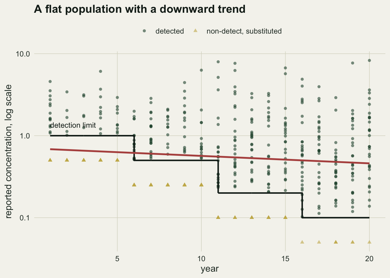
image-alt: "Log scale scatter against year over twenty years in a single panel, the vertical axis labelled 0.1, 1.0 and 10.0, with a black stepped detection limit that drops three times, from 1.0 down to 0.1, and yellow triangles marking the censored values below each step. The upper edge of the point cloud holds a similar height throughout while its lower edge steps down with the limit, and a red fitted line slopes gently downwards."
---
The laboratory returns "< 0.05". That is not a missing value, because the sample was measured and the measurement carries information: the concentration is somewhere between zero and 0.05. It is also not 0.05, and not 0.025, and not zero, although the spreadsheet will end up containing one of those three.
Substituting a number for a non-detect is the standard practice in nutrient chemistry, ecotoxicology, trace elements and qPCR, and it has two costs that are easy to miss. The first is bias in the summary statistics, and it runs in opposite directions for the mean and the spread. The second is worse and is the subject of most of this post: when the detection limit changes over the life of a monitoring programme, substitution manufactures a trend in a population that never moved.
## What substitution does to a summary
A lognormal concentration, one detection limit, four of the usual rules.
```{r setup}
#| message: false
#| warning: false
library(ggplot2)

te_paper  <- "#f5f4ee"
te_ink    <- "#16241d"
te_body   <- "#2c3a31"
te_forest <- "#275139"
te_rust   <- "#b5534e"
te_gold   <- "#c9b458"
te_line   <- "#dad9ca"

theme_datasheet <- function() {
  theme_minimal(base_size = 12) +
    theme(plot.background  = element_rect(fill = te_paper, colour = NA),
          panel.background = element_rect(fill = te_paper, colour = NA),
          panel.grid.major = element_line(colour = te_line, linewidth = 0.3),
          panel.grid.minor = element_blank(),
          text             = element_text(colour = te_body),
          plot.title       = element_text(colour = te_ink, face = "bold"),
          axis.text        = element_text(colour = te_body))
}

mu_log <- -0.6
sd_log <- 1.0

set.seed(20260806)
truth <- rlnorm(20000, mu_log, sd_log)
dl    <- 0.5

rules <- c(zero = 0, half = dl / 2, root2 = dl / sqrt(2), full = dl)
subst <- sapply(rules, function(v) ifelse(truth < dl, v, truth))

round(rbind(mean = c(true = mean(truth), apply(subst, 2, mean)),
            sd   = c(true = sd(truth),   apply(subst, 2, sd))), 3)
```
`r sprintf("%.0f", 100 * mean(truth < dl))` per cent of these samples are non-detects, which is ordinary for a trace analyte. The true mean is `r sprintf("%.3f", mean(truth))` and the true standard deviation `r sprintf("%.3f", sd(truth))`. Substituting zero pulls the mean down to `r sprintf("%.3f", mean(subst[, "zero"]))` and pushes the spread up to `r sprintf("%.3f", sd(subst[, "zero"]))`; substituting the full limit pushes the mean up to `r sprintf("%.3f", mean(subst[, "full"]))` and squeezes the spread down to `r sprintf("%.3f", sd(subst[, "full"]))`.
The mean and the standard deviation move in opposite directions, so no single substituted value gets both right. Half the limit happens to land close on the mean here, which is why it is the rule everyone uses, and it is close by coincidence of this distribution and this censoring fraction rather than by any property of the rule.
## The same programme, an improving laboratory
Now the case that matters. Twenty years of monitoring, thirty samples a year, and a concentration distribution that does not change at all. The only thing that changes is the laboratory: the detection limit drops from 1.0 to 0.5 to 0.2 to 0.1 across four five-year eras, because the instruments got better.
```{r series}
n_year  <- 30
years   <- 1:20
dl_era  <- c(rep(1.0, 5), rep(0.5, 5), rep(0.2, 5), rep(0.1, 5))

one_series <- function() {
  d <- data.frame(year = rep(years, each = n_year),
                  dl   = rep(dl_era, each = n_year))
  d$conc     <- rlnorm(nrow(d), mu_log, sd_log)     # never changes
  d$censored <- d$conc < d$dl
  d$reported <- ifelse(d$censored, d$dl / 2, d$conc)
  d
}

set.seed(14)
series <- one_series()
c(censored_overall = mean(series$censored),
  censored_era1    = mean(series$censored[series$year <= 5]),
  censored_era4    = mean(series$censored[series$year > 15]))
```
Over the whole record `r sprintf("%.0f", 100 * mean(series$censored))` per cent of samples are non-detects, but the fraction falls from `r sprintf("%.0f", 100 * mean(series$censored[series$year <= 5]))` per cent in the first era to `r sprintf("%.0f", 100 * mean(series$censored[series$year > 15]))` per cent in the last. That decline is real and it is a fact about the laboratory. The substituted value that stands in for those non-detects falls with it, from 0.5 to 0.05, and that is where the trend comes from.
```{r naive-trend}
naive <- lm(log(reported) ~ year, data = series)
round(coef(summary(naive)), 5)
```
The slope is `r sprintf("%.4f", coef(naive)[["year"]])` per year on the log scale, with p `r ifelse(coef(summary(naive))["year", "Pr(>|t|)"] < 0.001, "below 0.001", sprintf("= %.3f", coef(summary(naive))["year", "Pr(>|t|)"]))`. Over the twenty years that is a `r sprintf("%.1f", 100 * (1 - exp(coef(naive)[["year"]] * 19)))` per cent decline in a quantity that was drawn from the same distribution every single year.
```{r fig-series}
#| fig-cap: "One simulated twenty-year record. Detected values are shown as points, non-detects at the substituted half-limit, with the stepped detection limit and the fitted trend through the reported values."
#| fig-alt: "A scatter of concentrations on a log axis over twenty years, with a stepped line dropping three times marking the detection limit. The substituted non-detects form flat bands that step down with it, and a fitted line through all the reported values slopes clearly downwards while the detected points show no trend."
series$kind <- ifelse(series$censored, "non-detect, substituted", "detected")

ggplot(series, aes(x = year, y = reported)) +
  geom_point(aes(colour = kind, shape = kind), size = 1.5, alpha = 0.6) +
  geom_step(aes(y = dl), direction = "hv", linewidth = 0.9, colour = te_ink) +
  geom_smooth(method = "lm", formula = y ~ x, se = FALSE,
              linewidth = 1.1, colour = te_rust) +
  annotate("text", x = 1, y = 1.35, hjust = 0, size = 3.4, colour = te_ink,
           label = "detection limit") +
  scale_y_log10() +
  scale_colour_manual(values = c("detected" = te_forest,
                                 "non-detect, substituted" = te_gold)) +
  scale_shape_manual(values = c(16, 17)) +
  labs(x = "year", y = "reported concentration, log scale",
       colour = NULL, shape = NULL,
       title = "A flat population with a downward trend") +
  theme_datasheet() +
  theme(legend.position = "top")
```
## The likelihood that does not need a substituted value
A non-detect is an interval observation: the concentration is below the limit, and the probability of seeing that is the distribution function evaluated at the limit. Detected values contribute their density. Adding the two gives a likelihood that uses every sample without inventing a number for any of them, and it handles a limit that changes between samples without any extra machinery, because each observation carries its own limit.
The mechanics of interval-censored likelihoods are set out in the post on [rounded and coarsened measurements](../rounded-and-coarsened-measurements/); this is the one-sided case, where the lower edge of the interval is zero.
```{r censored-ml}
nll <- function(par, d) {
  m <- par[1] + par[2] * d$year
  s <- exp(par[3])
  ll <- ifelse(d$censored,
               plnorm(d$dl, m, s, log.p = TRUE),
               dlnorm(d$conc_obs, m, s, log = TRUE))
  -sum(ll)
}

series$conc_obs <- ifelse(series$censored, NA, series$conc)
fit_ml <- optim(c(mu_log, 0, log(sd_log)), nll, d = series,
                method = "BFGS", hessian = TRUE)
se_ml  <- sqrt(diag(solve(fit_ml$hessian)))[2]

round(c(slope = fit_ml$par[2], se = se_ml,
        lower = fit_ml$par[2] - 1.96 * se_ml,
        upper = fit_ml$par[2] + 1.96 * se_ml,
        sd = exp(fit_ml$par[3]), converged = fit_ml$convergence), 5)
```
The maximum likelihood slope is `r sprintf("%.5f", fit_ml$par[2])` per year with a standard error of `r sprintf("%.5f", se_ml)`, so the interval runs from `r sprintf("%.4f", fit_ml$par[2] - 1.96 * se_ml)` to `r sprintf("%.4f", fit_ml$par[2] + 1.96 * se_ml)` and sits squarely on the truth of zero. The recovered standard deviation on the log scale is `r sprintf("%.3f", exp(fit_ml$par[3]))` against a truth of `r sprintf("%.1f", sd_log)`. The same data that gave a `r sprintf("%.0f", 100 * (1 - exp(coef(naive)[["year"]] * 19)))` per cent decline gives no detectable trend once the non-detects are treated as what they are.
The two estimates use exactly the same observations. The difference is that one of them was told which values are bounds.
## How much censoring it takes
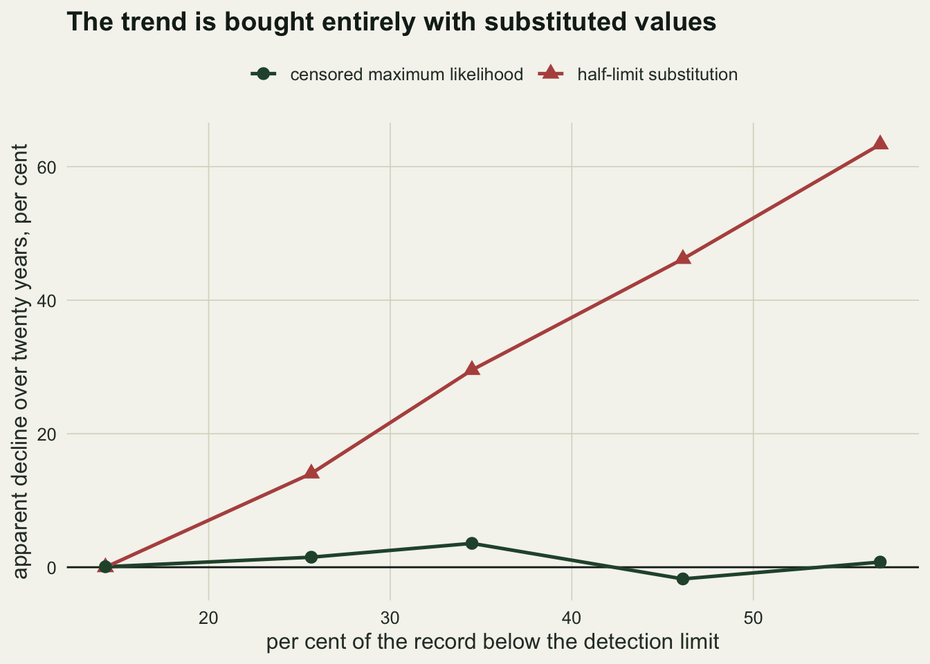
The size of the fabricated trend is a function of how much of the record is below the limit, so it is worth seeing the whole curve rather than one point on it.
```{r sweep}
sweep_dl <- function(scale_up, reps = 60) {
  out <- data.frame()
  for (k in scale_up) {
    res <- replicate(reps, {
      d <- one_series()
      d$dl <- d$dl * k
      d$censored <- d$conc < d$dl
      d$reported <- ifelse(d$censored, d$dl / 2, d$conc)
      d$conc_obs <- ifelse(d$censored, NA, d$conc)
      b_naive <- coef(lm(log(reported) ~ year, data = d))[["year"]]
      p_naive <- coef(summary(lm(log(reported) ~ year, data = d)))["year", "Pr(>|t|)"]
      f <- optim(c(mu_log, 0, log(sd_log)), nll, d = d, method = "BFGS")
      c(cens = mean(d$censored), naive = b_naive, ml = f$par[2],
        sig = p_naive < 0.05)
    })
    out <- rbind(out, data.frame(
      censored = mean(res["cens", ]),
      naive    = mean(res["naive", ]),
      ml       = mean(res["ml", ]),
      sig      = mean(res["sig", ]),
      decline  = 100 * (1 - exp(mean(res["naive", ]) * 19))))
  }
  out
}

set.seed(3)
sw <- sweep_dl(c(0.4, 0.7, 1.0, 1.5, 2.2))
round(sw, 4)
```
At `r sprintf("%.0f", 100 * sw$censored[1])` per cent censoring there is nothing to see: the fabricated decline is `r sprintf("%.1f", sw$decline[1])` per cent and the naive test calls it significant in `r sprintf("%.0f", 100 * sw$sig[1])` per cent of runs, which is the nominal five per cent to within the noise of sixty replicates. By `r sprintf("%.0f", 100 * sw$censored[2])` per cent it is a `r sprintf("%.1f", sw$decline[2])` per cent decline, significant `r sprintf("%.0f", 100 * sw$sig[2])` per cent of the time; at `r sprintf("%.0f", 100 * sw$censored[3])` per cent, which is roughly the record plotted above, `r sprintf("%.1f", sw$decline[3])` per cent and `r sprintf("%.0f", 100 * sw$sig[3])` per cent; and at `r sprintf("%.0f", 100 * sw$censored[nrow(sw)])` per cent, `r sprintf("%.1f", sw$decline[nrow(sw)])` per cent in every single run. The maximum likelihood slope stays within `r sprintf("%.4f", max(abs(sw$ml)))` of zero across the whole range.
The threshold worth remembering is the one between the first two rows. Somewhere around a quarter of the record being non-detect, substitution stops being a rounding convention and starts being the thing that produces the result.
```{r fig-sweep}
#| fig-cap: "Fabricated twenty-year decline from half-limit substitution against the fraction of the record below the limit, with the censored maximum likelihood estimate for comparison. Sixty simulated programmes per point."
#| fig-alt: "Two curves against the censored fraction. The substitution curve starts at zero at the lowest censoring and then climbs steeply to a large fabricated decline, while the maximum likelihood curve lies flat along the zero line across the whole range."
long <- rbind(
  data.frame(censored = sw$censored, decline = sw$decline,
             method = "half-limit substitution"),
  data.frame(censored = sw$censored,
             decline = 100 * (1 - exp(sw$ml * 19)),
             method = "censored maximum likelihood"))

ggplot(long, aes(x = 100 * censored, y = decline, colour = method,
                 shape = method)) +
  geom_hline(yintercept = 0, colour = te_ink, linewidth = 0.5) +
  geom_line(linewidth = 0.9) +
  geom_point(size = 2.9) +
  scale_colour_manual(values = c("half-limit substitution" = te_rust,
                                 "censored maximum likelihood" = te_forest)) +
  scale_shape_manual(values = c(16, 17)) +
  labs(x = "per cent of the record below the detection limit",
       y = "apparent decline over twenty years, per cent",
       colour = NULL, shape = NULL,
       title = "The trend is bought entirely with substituted values") +
  theme_datasheet() +
  theme(legend.position = "top")
```
## What to record and what to report
Keep the flag and the limit, not the substituted number. Two columns, one logical and one numeric, and the analysis can do anything it likes afterwards. A file that contains only `0.25` has destroyed the distinction between a measurement and a bound, and no later analysis can recover it.
Report the censoring fraction alongside any summary from censored data, because a mean from a record that is `r sprintf("%.0f", 100 * sw$censored[1])` per cent non-detect and one that is `r sprintf("%.0f", 100 * sw$censored[nrow(sw)])` per cent non-detect are not comparable quantities even when they carry the same units. And if the limit changed during the programme, say when and by how much, because that is a covariate whether or not anyone modelled it.
## Honest limits
The censored likelihood needs a distributional assumption where substitution needs none, and that is a real trade. Lognormal is conventional for concentrations and is what generated the data here, so this comparison is friendly to the method. A misspecified distribution biases the estimate in its own way, and the check is the usual one: fit an alternative family and see whether the conclusion moves. Non-parametric alternatives exist, Kaplan-Meier run on the reversed scale being the common one, and they carry less structure at the cost of less precision.
Very heavy censoring defeats everything. Past roughly three quarters non-detect there is little left to identify the lower tail with, and the honest report is the detection frequency itself rather than a mean nobody can estimate.
This is censoring, not truncation. A non-detect is present in the record with partial information; a truncated observation is absent altogether, which is a different problem with a different fix, treated in the post on [truncated parasite burdens](../truncated-parasite-burden/).
The detection limit is itself an estimate, it varies between batches and matrices, and laboratories do not always report the value they actually used. Where the limit is uncertain the interval is wider than modelled here, and the fabricated trend above is a lower bound on what a changing limit can do.
Finally, the mechanism is not confined to detection limits. Any bound that moves during a monitoring programme does the same thing: a reporting threshold, a minimum countable size, a changed survey protocol. The [post on splicing a monitoring series](../splicing-a-monitoring-series/) treats the version where a method change puts a step in the mean; here an unchanged population acquires a slope.
## References
Helsel DR 2006 Chemosphere 65(11):2434-2439 (10.1016/j.chemosphere.2006.04.051)
Shoari N, Dube JS 2018 Environmental Toxicology and Chemistry 37(3):643-656 (10.1002/etc.4046)
Helsel DR 2012 Statistics for Censored Environmental Data Using Minitab and R, 2nd edition, Wiley, ISBN 978-0-470-47988-9
## Related tutorials
- [Rounded and coarsened measurements](../rounded-and-coarsened-measurements/)
- [Truncated parasite burdens](../truncated-parasite-burden/)
- [Faecal egg count reduction tests at low counts](../faecal-egg-count-reduction-test/)
- [Compositional analysis and zeros](../compositional-analysis-and-zeros/)