library(ggplot2)
clr <- function(x) { lx <- log(x); lx - mean(lx) }
te_ink <- "#16241d"; te_forest <- "#275139"; te_faint <- "#5d6b61"
te_paper <- "#f5f4ee"; te_line <- "#dad9ca"; te_red <- "#b5534e"
theme_te <- function(base = 12) theme_minimal(base_size = base) + theme(
  plot.background = element_rect(fill = te_paper, colour = NA),
  panel.background = element_rect(fill = te_paper, colour = NA),
  panel.grid.major = element_line(colour = te_line, linewidth = 0.3),
  panel.grid.minor = element_blank(),
  axis.text = element_text(colour = "#2c3a31"), axis.title = element_text(colour = te_ink),
  plot.title = element_text(colour = te_ink, face = "bold"),
  plot.subtitle = element_text(colour = te_faint, size = rel(0.9)),
  legend.position = "top")
theme_set(theme_te())Compositional analysis and the zero problem
R
compositional data
ggplot2
simulation
ecology tutorial
How closure turns one real change into many spurious ones, why log-ratios localise it correctly, and how to handle the zeros that log-ratios cannot take.
Corrected 27 September 2026: a zero for a rare taxon is now described as a sampling zero or a value below a detection limit, not as a detection-limit value in every case; the title of the false-positive figure said closure made six spurious changes and now says five, since one of the six flagged taxa really did change.
The first two posts built the machinery: closure distorts correlation and distance, and the log-ratio transformations repair it. This post puts the machinery to work on the question ecologists actually ask, which taxa differ between two groups, and shows why the naive answer is usually wrong. It then confronts the one obstacle that stands between compositional theory and real sequencing or count data: log-ratios are undefined when a count is zero, and zeros are everywhere.
Setup
One change, many false positives
We build a two-group comparison where the truth is under our control. Six taxa; between control and treatment, only taxon one changes in absolute abundance, a 2.6-fold increase. The other five are identical in absolute terms. Then we close to proportions, as any pipeline would, and run the standard per-taxon test on each proportion.
set.seed(4472)
D <- 6L; ng <- 60L
base_mu <- c(3.4, 2.6, 2.4, 2.2, 2.0, 2.3); sd_log <- rep(0.45, D)
delta1  <- log(2.6)                              # taxon 1 rises; taxa 2..6 unchanged
sim_abs <- function(mu) sapply(1:D, function(j) rlnorm(ng, mu[j], sd_log[j]))
Xc <- sim_abs(base_mu)
mu_t <- base_mu; mu_t[1] <- mu_t[1] + delta1
Xt <- sim_abs(mu_t)
Pc <- Xc / rowSums(Xc); Pt <- Xt / rowSums(Xt)

p_raw <- sapply(1:D, function(j) t.test(Pc[,j], Pt[,j])$p.value)
setNames(round(p_raw, 6), paste0("t", 1:D))
t1 t2 t3 t4 t5 t6
0.000000 0.000003 0.000012 0.000576 0.000266 0.000000 The test flags all 6 taxa as significantly different, taxon one at \(1.4 \times 10^{-18}\) and even the least affected unchanged taxon at \(5.8 \times 10^{-4}\). Yet five of the six did not change at all. Closure is the culprit: when taxon one takes up more of the total, every other proportion is pushed down, whether or not its absolute abundance moved. The naive analysis cannot tell a real change from its shadow.
dfp <- data.frame(taxon = factor(1:D), nl = -log10(p_raw),
                  truth = ifelse(1:D == 1, "truly changed (absolute)", "unchanged (absolute)"))
p_falsepos <- ggplot(dfp, aes(taxon, nl, fill = truth)) +
  geom_col(width = 0.65) +
  geom_hline(yintercept = -log10(0.05), linetype = "dashed", colour = te_faint) +
  scale_fill_manual(values = c("truly changed (absolute)" = te_forest,
                               "unchanged (absolute)" = te_red), name = NULL) +
  labs(title = "Closure turns one real change into five spurious ones",
       subtitle = "Only taxon 1 changed; the naive proportion test flags every taxon",
       x = "taxon", y = "naive proportion test  (-log10 p)")
p_falsepos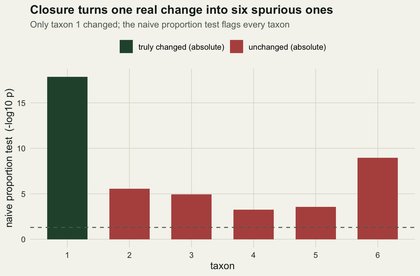
The log-ratio view localises the change correctly. The ratios among the five unchanged taxa are untouched, because both parts of each ratio held still; only ratios that involve taxon one move.
pairs <- t(combn(1:D, 2))
p_lr <- apply(pairs, 1, function(pr) {
  t.test(log(Xc[,pr[1]] / Xc[,pr[2]]), log(Xt[,pr[1]] / Xt[,pr[2]]))$p.value })
has1 <- apply(pairs, 1, function(pr) 1 %in% pr)
c(among_unchanged_sig = sum(p_lr[!has1] < 0.05), of = sum(!has1),
  involving_t1_sig     = sum(p_lr[has1] < 0.05),  of_ = sum(has1))
among_unchanged_sig of involving_t1_sig of_
0 10 5 5 None of the 10 ratios among the unchanged taxa is significant, and all 5 ratios involving taxon one are. The signal is where it belongs. To confirm this is not luck, we can repeat the whole simulation and record the false-positive rate on the unchanged taxa under each approach.
set.seed(55)
B <- 1500L
mc <- replicate(B, {
  a <- sim_abs(base_mu); mt <- base_mu; mt[1] <- mt[1] + delta1; b <- sim_abs(mt)
  pa <- a / rowSums(a); pb <- b / rowSums(b)
  pr_raw <- sapply(2:D, function(j) t.test(pa[,j], pb[,j])$p.value)
  prs <- t(combn(2:D, 2))
  pr_lr <- apply(prs, 1, function(pr) t.test(log(a[,pr[1]]/a[,pr[2]]), log(b[,pr[1]]/b[,pr[2]]))$p.value)
  c(raw = mean(pr_raw < 0.05), lr = mean(pr_lr < 0.05))
})
round(c(naive_proportion = mean(mc["raw",]), coda_logratio = mean(mc["lr",])), 3)
naive_proportion coda_logratio
0.999 0.051 The naive proportion test wrongly flags an unchanged taxon 99.9 per cent of the time; the log-ratio test holds at 0.051, the nominal rate. This is the reason differential-abundance methods for sequencing data work on log-ratios rather than proportions.
Ordination sees the same distortion
Principal component analysis inherits the problem. On raw proportions the first axis is dominated by the abundant, closure-driven part; on clr coordinates the variance spreads across axes that reflect ratios.
P <- rbind(Pc, Pt); CLR <- t(apply(P, 1, clr))
vr_raw <- summary(prcomp(P,   center = TRUE))$importance[2, 1:2]
vr_clr <- summary(prcomp(CLR, center = TRUE))$importance[2, 1:2]
round(rbind(raw_proportions = vr_raw, clr = vr_clr), 3)
PC1 PC2
raw_proportions 0.745 0.100
clr 0.327 0.203The first raw-proportion axis absorbs 75 per cent of the variance against 33 per cent for clr. A single dominant axis on proportions looks like clean structure but is largely the closure artefact; the clr ordination distributes variance across the ratios that carry the ecology.
The zero problem
Everything above assumed strictly positive parts. Real count data violate that constantly: a rare taxon is simply not seen in a given sample, and its count is zero. A logarithm of zero is undefined, so a single zero breaks every log-ratio in that sample. We generate counts by drawing per-sample compositions and sampling reads at modest depth, which produces exactly this.
set.seed(6190)
Dz <- 6L; nz <- 80L
rel_mu <- c(0.30, 0.24, 0.20, 0.14, 0.10, 0.02)     # taxon 6 genuinely rare
Comp <- t(apply(matrix(rgamma(nz * Dz, rep(rel_mu * 40, each = nz)), nz, Dz), 1,
                function(z) z / sum(z)))
Nlib <- sample(120:180, nz, replace = TRUE)
Counts <- t(sapply(1:nz, function(i) rmultinom(1, Nlib[i], Comp[i,])[,1]))

nz_cells <- Counts == 0
c(zero_cells = sum(nz_cells), of = nz * Dz,
  rare_taxon_zero_in = sum(nz_cells[,6]), samples = nz)
zero_cells of rare_taxon_zero_in samples
22 480 21 80 Here 22 of 480 cells are zero, and the rare taxon is absent from 21 of 80 samples. Attempting the clr on such a sample returns non-finite values, and the analysis stops.
any(!is.finite(clr((Counts / rowSums(Counts))[which(nz_cells[,6])[1], ])))[1] TRUEReplacing zeros, and the choice it hides
The standard remedy is multiplicative replacement: put a small positive value in each zero and scale the observed parts down so the composition still sums to one. Done multiplicatively, this preserves the ratios among the parts that were actually observed.
mult_repl <- function(cnt, delta) {
  p <- cnt / sum(cnt); z <- p == 0; k <- sum(z)
  if (k == 0) return(p)
  p[z] <- delta; p[!z] <- p[!z] * (1 - k * delta); p
}
i0 <- which(nz_cells[,6])[1]
c(observed_ratio_small_delta = log(mult_repl(Counts[i0,], 0.2 / Nlib[i0])[1] /
                                    mult_repl(Counts[i0,], 0.2 / Nlib[i0])[2]),
  observed_ratio_large_delta = log(mult_repl(Counts[i0,], 1.0 / Nlib[i0])[1] /
                                    mult_repl(Counts[i0,], 1.0 / Nlib[i0])[2]),
  rare_ratio_small_delta     = log(mult_repl(Counts[i0,], 0.2 / Nlib[i0])[6] /
                                    mult_repl(Counts[i0,], 0.2 / Nlib[i0])[1]),
  rare_ratio_large_delta     = log(mult_repl(Counts[i0,], 1.0 / Nlib[i0])[6] /
                                    mult_repl(Counts[i0,], 1.0 / Nlib[i0])[1]))
observed_ratio_small_delta observed_ratio_large_delta
0.6241543 0.6241543
rare_ratio_small_delta rare_ratio_large_delta
-5.6336590 -4.0196860 The ratio between two observed taxa is identical for the two replacement values, to machine precision. The ratio that involves the previously-zero taxon is not: it swings by more than 1.6 on the log scale as the imputed value changes. In other words, any conclusion about the rare taxon is a conclusion about the number we chose to put in its place. A sweep across replacement sizes makes this visible.
deltas <- c(0.1, 0.2, 0.35, 0.5, 0.65, 0.8, 1.0)
mclr6 <- sapply(deltas, function(dd) {
  Pr <- t(sapply(1:nz, function(i) mult_repl(Counts[i,], dd / Nlib[i]))); mean(t(apply(Pr,1,clr))[,6]) })
mlr12 <- sapply(deltas, function(dd) {
  Pr <- t(sapply(1:nz, function(i) mult_repl(Counts[i,], dd / Nlib[i]))); mean(log(Pr[,1] / Pr[,2])) })
dz <- rbind(data.frame(delta = deltas, val = mclr6, series = "clr of rare taxon (was zero)"),
            data.frame(delta = deltas, val = mlr12, series = "log-ratio of two common taxa"))
ggplot(dz, aes(delta, val, colour = series)) +
  geom_line(linewidth = 0.9) + geom_point(size = 2) +
  scale_colour_manual(values = c("clr of rare taxon (was zero)" = te_red,
                                 "log-ratio of two common taxa" = te_forest), name = NULL) +
  labs(title = "The zero replacement is an untestable choice",
       subtitle = "Observed ratios are invariant; the rare-taxon value tracks the imputed delta",
       x = "imputed value delta  (units of 1/N)", y = "mean log-ratio quantity")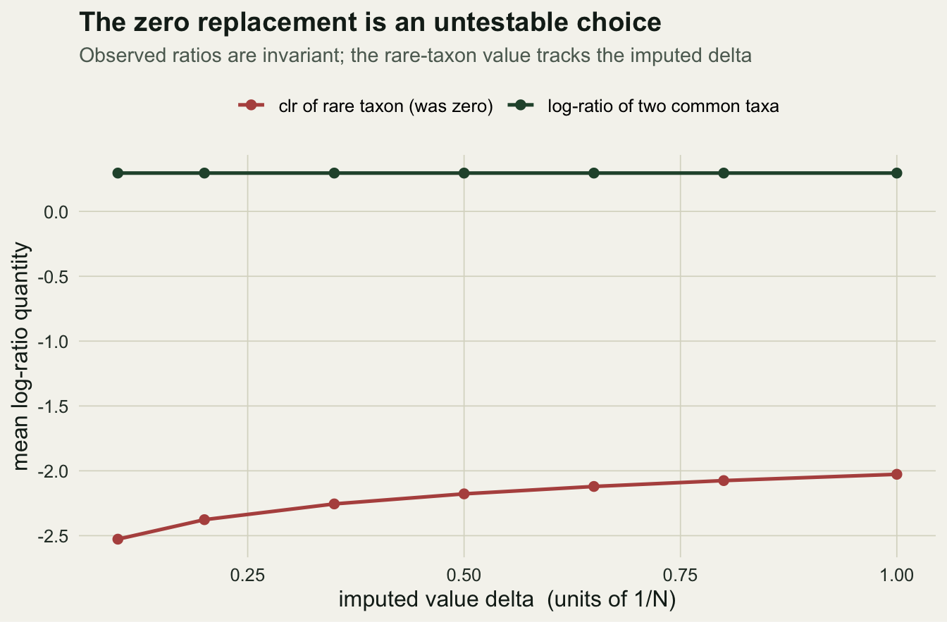
The mean rare-taxon clr moves by 0.5 across the range of replacement values. A more principled version replaces each zero with a Dirichlet posterior expectation rather than a flat constant, but a prior is still a choice: a Jeffreys prior and a uniform prior give visibly different rare-taxon values.
bayes_repl <- function(cnt, a) (cnt + a) / (sum(cnt) + length(cnt) * a)
c(dirichlet_half = mean(sapply(1:nz, function(i) clr(bayes_repl(Counts[i,], 0.5))[6])),
  dirichlet_one  = mean(sapply(1:nz, function(i) clr(bayes_repl(Counts[i,], 1.0))[6])))
dirichlet_half dirichlet_one
-2.081182 -1.856665 The honest limit, and a bridge
Two limits sit under this post. The first is the one carried through the whole series: log-ratios answer relative questions. A taxon that rises in relative abundance may be flat or falling in absolute terms if the total moved, and the composition alone cannot say which. The second is specific to zeros. A count of zero for a rare taxon is a sampling zero or a value below a detection limit, not necessarily a true absence, and replacing it is imputation under an assumption that the data cannot check. That is the same predicament as elsewhere in statistics: a missing value has to be filled with something, and the fill rests on a belief about what would have been there. Readers who have worked through the missing-data series will recognise the shape of it. The next and final post makes both limits quantitative and shows how to check whether a compositional conclusion depends on them.
What comes next
The closing post of the series is a set of checks: does a naive verdict survive dropping a part, do the model residuals behave, and, most importantly, how far can an absolute claim be pushed before the unmeasured total overturns it. That last check turns the honest limit into a single number a reader can argue with.
References
Aitchison J 1983 Biometrika 70(1):57-65 (10.1093/biomet/70.1.57)
Martin-Fernandez JA, Barcelo-Vidal C, Pawlowsky-Glahn V 2003 Mathematical Geology 35(3):253-278 (10.1023/A:1023866030544)
Palarea-Albaladejo J, Martin-Fernandez JA 2015 Chemometrics and Intelligent Laboratory Systems 143:85-96 (10.1016/j.chemolab.2015.02.019)
Gloor GB, Macklaim JM, Pawlowsky-Glahn V, Egozcue JJ 2017 Frontiers in Microbiology 8:2224 (10.3389/fmicb.2017.02224)
Lin H, Peddada SD 2020 Nature Communications 11:3514 (10.1038/s41467-020-17041-7)