library(ggplot2)
clr <- function(x) { lx <- log(x); lx - mean(lx) }          # centred log-ratio
alr <- function(x, ref = length(x)) log(x[-ref] / x[ref])   # additive log-ratio
C   <- function(x) x / sum(x)                                # closure
ilr_basis <- function(D) {                                  # orthonormal contrast matrix
  V <- matrix(0, D, D - 1)
  for (i in seq_len(D - 1)) {
    a <- sqrt(1 / (i * (i + 1))); b <- sqrt(i / (i + 1))
    V[1:i, i] <- a; V[i + 1, i] <- -b
  }
  V
}
te_ink <- "#16241d"; te_forest <- "#275139"; te_faint <- "#5d6b61"
te_paper <- "#f5f4ee"; te_line <- "#dad9ca"; te_red <- "#b5534e"
theme_te <- function(base = 12) theme_minimal(base_size = base) + theme(
  plot.background = element_rect(fill = te_paper, colour = NA),
  panel.background = element_rect(fill = te_paper, colour = NA),
  panel.grid.major = element_line(colour = te_line, linewidth = 0.3),
  panel.grid.minor = element_blank(),
  axis.text = element_text(colour = "#2c3a31"), axis.title = element_text(colour = te_ink),
  plot.title = element_text(colour = te_ink, face = "bold"),
  plot.subtitle = element_text(colour = te_faint, size = rel(0.9)), legend.position = "top")
theme_set(theme_te())

set.seed(3390)
D <- 5L; n <- 300L
mu <- c(2.8, 2.4, 2.0, 1.6, 2.2); sdlog <- c(0.5, 0.6, 0.55, 0.7, 0.5)
X <- sapply(1:D, function(j) rlnorm(n, mu[j], sdlog[j]))
P <- X / rowSums(X)
V <- ilr_basis(D)Log-ratio transformations: clr, alr and ilr
R
compositional data
ggplot2
ecology tutorial
Building the centred, additive and isometric log-ratio transformations by hand, with Aitchison distance, perturbation and powering, using base R only.
Corrected 27 September 2026: the post said the ilr coordinates are uncorrelated by construction; what is orthonormal is the basis, and the coordinates computed on it are not in general uncorrelated across samples.
The previous post showed that proportions carry a constant-sum constraint that manufactures negative correlations and makes ordinary correlation subcompositionally incoherent. The one quantity that behaved well was the log-ratio. This post takes that hint seriously and builds the three standard log-ratio transformations from first principles: the centred log-ratio, the additive log-ratio, and the isometric log-ratio. Each maps a composition off the constrained simplex and into ordinary Euclidean space, where distance, correlation and ordination recover their usual meaning. All three are a few lines of base R.
Setup
The centred log-ratio
The centred log-ratio takes logarithms of the parts and subtracts their mean, which is the same as dividing every part by the geometric mean of the composition. The result is a vector that sums to zero.
CLR <- t(apply(P, 1, clr))
max(abs(rowSums(CLR)))       # rows sum to zero
[1] 1.110223e-15The rows sum to zero; the tiny printed value is floating-point rounding. That zero-sum property is exactly what makes the clr convenient and what makes it awkward. Convenient, because clr coordinates live in ordinary space and each one is interpretable as a part against the average part. Awkward, because the zero-sum means the coordinates are linearly dependent: their covariance matrix is singular and cannot be inverted.
ev <- eigen(cov(CLR), only.values = TRUE)$values
c(smallest_eigenvalue = min(abs(ev)), rank = qr(cov(CLR))$rank, parts = D)
smallest_eigenvalue rank parts
1.440082e-16 4.000000e+00 5.000000e+00 The smallest eigenvalue is zero up to floating-point rounding (the printed value above) and the matrix has rank 4 for 5 parts. Any method that needs a full-rank covariance, discriminant analysis or a multivariate normal likelihood among them, cannot take clr coordinates directly. That is what the isometric log-ratio fixes.
A picture of the simplex
Before the algebra, a picture helps. A three-part composition is a point in a triangle: the three corners are the pure compositions, and every interior point is a mixture. Distances and directions in this triangle are not the ordinary ones. The natural operations are perturbation, which plays the role of a translation, and powering, which plays the role of scaling. Perturbation of one composition by another is the closed elementwise product; powering is the closed elementwise power.
set.seed(11)
A3 <- sapply(1:3, function(j) rlnorm(9, c(2.2, 2.0, 1.6)[j], 0.5)); T3 <- A3 / rowSums(A3)
tern <- function(m) data.frame(tx = m[,2] + 0.5 * m[,3], ty = (sqrt(3)/2) * m[,3])
pts <- tern(T3)
vert <- data.frame(tx = c(0, 1, 0.5), ty = c(0, 0, sqrt(3)/2), lab = c("part A", "part B", "part C"))
edge <- data.frame(x = c(0, 1, 0.5), y = c(0, 0, sqrt(3)/2),
                   xend = c(1, 0.5, 0), yend = c(0, sqrt(3)/2, 0))
xstar <- C(T3[1,]); yv <- C(c(1.8, 1.0, 1.0)); xp <- C(xstar * yv)
pth <- tern(rbind(xstar, xp))
p_simplex <- ggplot() +
  geom_segment(data = edge, aes(x, y, xend = xend, yend = yend), colour = te_line, linewidth = 0.6) +
  geom_point(data = pts, aes(tx, ty), colour = te_forest, size = 2.2, alpha = 0.8) +
  geom_segment(data = data.frame(x = pth$tx[1], y = pth$ty[1], xend = pth$tx[2], yend = pth$ty[2]),
               aes(x, y, xend = xend, yend = yend), colour = te_red, linewidth = 0.9,
               arrow = arrow(length = unit(0.18, "cm"), type = "closed")) +
  geom_text(data = vert, aes(tx, ty, label = lab), vjust = c(1.6, 1.6, -0.8), colour = te_ink, size = 3.4) +
  coord_equal() + theme_void() +
  theme(plot.background = element_rect(fill = te_paper, colour = NA),
        plot.title = element_text(colour = te_ink, face = "bold"),
        plot.subtitle = element_text(colour = te_faint, size = rel(0.9))) +
  labs(title = "The simplex: sample space of compositions",
       subtitle = "Points are three-part compositions; the arrow is a perturbation")
p_simplex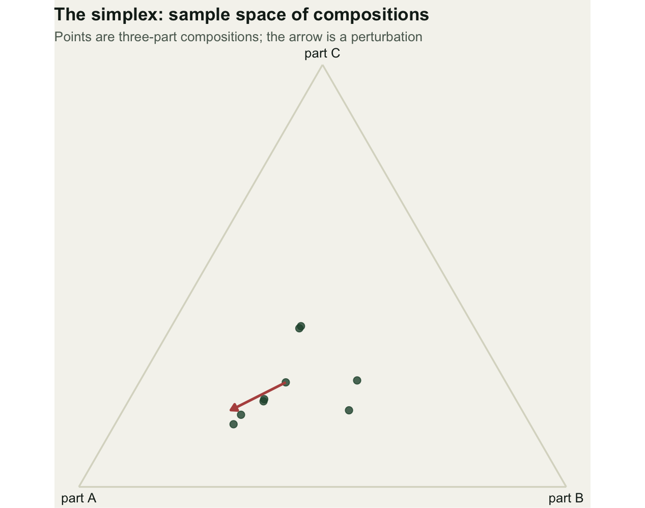
These operations are not exotic once viewed through the clr. Perturbation becomes ordinary addition, and powering becomes ordinary multiplication, in clr space.
y <- P[3, ]; a <- 2.3; xa <- P[1, ]
c(perturbation = max(abs(clr(C(xa * y)) - (clr(xa) + clr(y)))),
  powering     = max(abs(clr(C(xa^a)) - a * clr(xa))))
perturbation powering
2.220446e-16 4.440892e-16 Both identities hold to machine precision. The simplex, with perturbation and powering, is a vector space, and the clr is the map that turns its geometry into the geometry we already know.
Distance that respects ratios
The distance attached to this geometry is the Aitchison distance. It can be written three ways that all agree: as the ordinary distance between clr vectors, as the ordinary distance between isometric log-ratio vectors, and as a sum over all pairwise log-ratios. Computing one composition against another confirms the identity.
xa <- P[1, ]; xb <- P[2, ]
d_clr <- sqrt(sum((clr(xa) - clr(xb))^2))                 # Euclidean on clr
d_ilr <- sqrt(sum(((clr(xa) - clr(xb)) %*% V)^2))         # Euclidean on ilr
Lr <- function(x) outer(1:D, 1:D, function(i, j) log(x[i] / x[j]))
d_lr <- sqrt(sum((Lr(xa) - Lr(xb))^2) / (2 * D))          # pairwise log-ratio form
round(c(clr = d_clr, ilr = d_ilr, pairwise = d_lr), 5)
clr ilr pairwise
1.35279 1.35279 1.35279 All three give 1.353. This distance ranks pairs of samples very differently from ordinary Euclidean distance on the raw proportions. Euclidean distance is dominated by the abundant parts, so two samples that differ only in a rare taxon look almost identical even when that taxon changed by an order of magnitude. Aitchison distance weighs the ratios and sees the change.
CLRfull <- t(apply(P, 1, clr))
Draw <- as.matrix(dist(P)); Dait <- as.matrix(dist(CLRfull)); ut <- upper.tri(Draw)
rho <- cor(Draw[ut], Dait[ut], method = "spearman")
set.seed(9); s <- sample(which(ut), 3000)
ggplot(data.frame(euc = Draw[s], ait = Dait[s]), aes(euc, ait)) +
  geom_point(colour = te_forest, alpha = 0.25, size = 0.9) +
  labs(title = "Naive Euclidean distance is not Aitchison distance",
       subtitle = sprintf("Spearman rank agreement %.2f over all pairs", rho),
       x = "Euclidean distance on raw proportions", y = "Aitchison distance (Euclidean on clr)")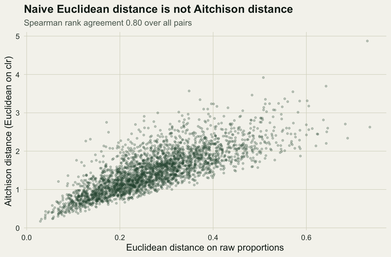
The Spearman rank agreement between the two distance matrices is 0.798. As one example, among the 44,850 pairs there is one that ranks 2161 of 44,850 by Euclidean distance, near the closest, yet ranks 41,119 by Aitchison distance, near the farthest. The two samples look almost the same in proportions but have very different internal ratios.
Additive and isometric coordinates
The additive log-ratio divides every part by a chosen reference part and takes logarithms. It gives 4 coordinates and is simple, but it is not isometric: distances measured on alr coordinates do not equal Aitchison distance, and they depend on which part was chosen as the reference.
d_alr <- sqrt(sum((alr(xa, 5) - alr(xb, 5))^2))
round(c(alr_euclidean = d_alr, aitchison = d_clr), 5)
alr_euclidean aitchison
1.92256 1.35279 The alr distance here is 1.923 against an Aitchison distance of 1.353. They differ, and a different reference would give a different alr distance. For interpreting a single contrast against a fixed baseline the alr is fine; for anything that relies on distances or angles it distorts them.
The isometric log-ratio removes that distortion. It projects the clr onto an orthonormal basis of the zero-sum space, giving 4 coordinates, one per degree of freedom with none redundant, that preserve Aitchison distance exactly. Orthonormality is a property of the basis: the coordinates computed on it are not in general uncorrelated across samples. The basis used here contrasts the geometric mean of the first i parts against part i + 1, scaled so that the columns are orthonormal.
c(orthonormal = max(abs(crossprod(V) - diag(D - 1))),
  reconstruct = max(abs(CLRfull - (CLRfull %*% V) %*% t(V))))
orthonormal reconstruct
2.220446e-16 6.661338e-16 The basis satisfies V'V = I to machine precision, and applying it and its transpose recovers the clr exactly. The ilr coordinates are the ones to feed to a discriminant analysis, a distance-based ordination, or a multivariate normal model, because they are full rank and isometric.
The honest limit
Each transformation trades one inconvenience for another. The clr is interpretable part by part but singular, so it cannot go into a method that inverts a covariance. The alr is simple but reference-dependent and non-isometric. The ilr is full rank and isometric but its coordinates are not individually interpretable: only the whole geometry means something, and a different orthonormal basis gives different coordinate values for the same distances. None of this recovers absolute abundance. Every log-ratio describes parts relative to one another, and the total that closure removed stays gone. Only two of the three agree on distances: the clr and the ilr give the same geometry and differ in how readable their coordinates are, while the alr gives neither the same distance nor a reference-free answer. The right choice depends on the question, not on which is best in the abstract.
What comes next
With coordinates that behave, the standard toolkit opens up: principal components on clr, clustering on Aitchison distance, and tests on balances. The next post applies these to a two-group comparison, shows how a single real change becomes many spurious ones under naive proportion tests, and confronts the practical obstacle that log-ratios cannot handle a zero.
References
Aitchison J 1982 Journal of the Royal Statistical Society: Series B (Methodological) 44(2):139-160 (10.1111/j.2517-6161.1982.tb01195.x)
Aitchison J 1986 The Statistical Analysis of Compositional Data. Monographs on Statistics and Applied Probability. Chapman and Hall, London. ISBN 978-0-412-28060-3
Egozcue JJ, Pawlowsky-Glahn V, Mateu-Figueras G, Barcelo-Vidal C 2003 Mathematical Geology 35(3):279-300 (10.1023/A:1023818214614)
Egozcue JJ, Pawlowsky-Glahn V 2005 Mathematical Geology 37(7):795-828 (10.1007/s11004-005-7381-9)
Pawlowsky-Glahn V, Egozcue JJ, Tolosana-Delgado R 2015 Modeling and Analysis of Compositional Data. Wiley, Chichester. ISBN 978-1-118-44306-4
Filzmoser P, Hron K, Templ M 2018 Applied Compositional Data Analysis: With Worked Examples in R. Springer, Cham. ISBN 978-3-319-96420-1