library(ggplot2)
clr <- function(x) { lx <- log(x); lx - mean(lx) }   # centred log-ratio
C   <- function(x) x / sum(x)                          # closure to the simplex

te_ink <- "#16241d"; te_forest <- "#275139"; te_faint <- "#5d6b61"
te_paper <- "#f5f4ee"; te_line <- "#dad9ca"; te_red <- "#b5534e"
theme_te <- function(base = 12) theme_minimal(base_size = base) + theme(
  plot.background = element_rect(fill = te_paper, colour = NA),
  panel.background = element_rect(fill = te_paper, colour = NA),
  panel.grid.major = element_line(colour = te_line, linewidth = 0.3),
  panel.grid.minor = element_blank(),
  axis.text = element_text(colour = "#2c3a31"), axis.title = element_text(colour = te_ink),
  plot.title = element_text(colour = te_ink, face = "bold"),
  plot.subtitle = element_text(colour = te_faint, size = rel(0.9)),
  strip.text = element_text(colour = te_ink, face = "bold"), legend.position = "top")
theme_set(theme_te())Closure and spurious correlation
R
compositional data
ggplot2
ecology tutorial
Why dividing counts by their total invents negative correlations between species that were independent, and why Pearson correlation on proportions misleads.
Ecologists rarely observe absolute abundances. A pitfall count, a sequencing run, a point count of a bird community: each gives numbers whose total depends on sampling effort, library size, or survey length as much as on the community itself. The usual reflex is to divide by the row total and work with proportions, so that samples become comparable. That single step, called closure, changes the correlation structure of the data in a way that is easy to miss and hard to undo.
This post shows the problem with a simulation where the truth is known: five taxa whose absolute abundances are statistically independent. After closure they look strongly, and misleadingly, associated. We then isolate the two properties of proportions that cause the trouble, and point to the transformation that repairs them. This is the first post in a short series on compositional data; the repair itself is the subject of the next one.
Setup
Everything here uses base R and ggplot2 only. The helper clr (the centred log-ratio) and C (closure) return later in the series; for now the palette and theme keep the figures consistent with the rest of the site.
Independent parts, invented correlation
We draw absolute abundances for five taxa from independent log-normal distributions. Nothing links them: taxon one carries no information about taxon two. The absolute correlations confirm it.
set.seed(8241)
n <- 500L; D <- 5L
mu    <- c(3.0, 2.6, 2.2, 1.8, 2.4)
sdlog <- c(0.55, 0.60, 0.50, 0.70, 0.58)
X <- sapply(seq_len(D), function(j) rlnorm(n, mu[j], sdlog[j]))   # absolute abundances
colnames(X) <- paste0("t", 1:D)

Cabs <- cor(X)
off_abs <- Cabs[upper.tri(Cabs)]
c(mean_abs_cor = mean(abs(off_abs)), max_abs_cor = max(abs(off_abs)))
mean_abs_cor max_abs_cor
0.03092436 0.06434976 The mean absolute correlation among the ten pairs is 0.031, the largest 0.064. These are the small correlations sampling noise produces from independent data.
Now close each row to proportions, exactly as one would before an ordination or a proportion barplot.
P <- X / rowSums(X)          # proportions: each row sums to 1
Cclo <- cor(P)
off_clo <- Cclo[upper.tri(Cclo)]
c(all_negative = all(off_clo < 0), mean_closed_cor = mean(off_clo),
  cor_t1_t2 = Cclo[1, 2])
all_negative mean_closed_cor cor_t1_t2
1.0000000 -0.2356567 -0.4818566 Every one of the ten pairwise correlations is now negative, with a mean of -0.236. The pair of taxa that were essentially uncorrelated in absolute terms, 0.011, correlate at -0.482 once closed. No biology has changed. The row total, a nuisance quantity, was removed, and the removal manufactured association.
d_abs <- data.frame(x = scale(log(X[,1])), y = scale(log(X[,2])),
                    space = "Absolute abundance (independent)")
d_clo <- data.frame(x = P[,1], y = P[,2], space = "Closed to proportions")
fp <- rbind(d_abs, setNames(d_clo, names(d_abs)))
p_closure <- ggplot(fp, aes(x, y)) +
  geom_point(colour = te_forest, alpha = 0.35, size = 1.1) +
  geom_smooth(method = "lm", se = FALSE, colour = te_red, linewidth = 0.9, formula = y ~ x) +
  facet_wrap(~ space, scales = "free") +
  labs(title = "Closure manufactures correlation",
       subtitle = "Parts are independent in absolute terms; the row total forces a negative tilt",
       x = "taxon 1", y = "taxon 2")
p_closure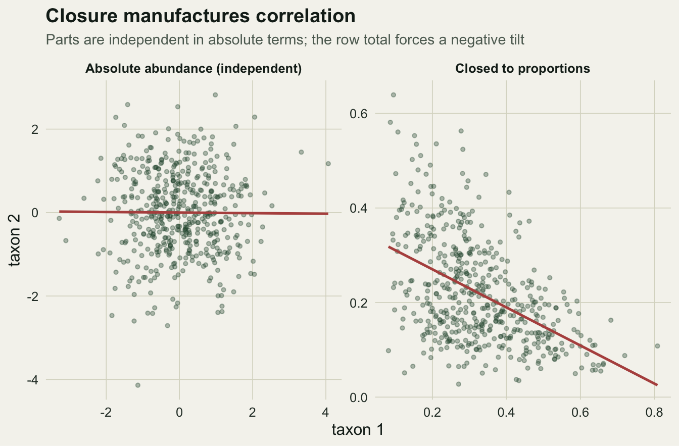
The constant-sum constraint
The negative correlations are not bad luck. They are forced by arithmetic. If the parts of every sample sum to one, their total has zero variance, and the covariance of any part with the sum of all parts must be zero. Writing that out, the covariances in each row of the covariance matrix are obliged to cancel.
S <- cov(P)
max(abs(rowSums(S)))     # each row of the covariance matrix sums to zero
[1] 1.517883e-17The printed maximum is zero up to floating-point rounding, so each row sums to zero. Because the off-diagonal entries of any row must offset a positive variance on the diagonal, at least some of them are pushed negative. With 5 parts the average pairwise correlation lands near the equal-variance value of minus one over 4, which is -0.25. A negative correlation between two proportions is therefore the default expectation, not evidence of competition or any other ecological process.
Subcompositional incoherence
There is a second, subtler failure. Suppose a reviewer asks you to drop the two rarest taxa and re-analyse the three that remain. You re-close the retained parts and recompute the correlation between taxa one and two. It changes.
sub <- X[, 1:3] / rowSums(X[, 1:3])     # subcomposition of taxa 1, 2, 3
c(full = cor(P[,1], P[,2]), sub = cor(sub[,1], sub[,2]))
full sub
-0.4818566 -0.7668225 In the full five-part composition the correlation is -0.482; in the three-part subcomposition it is -0.767. Same two taxa, same samples, a different number because the other parts were removed. A measure of association that depends on which unrelated parts happen to be in the table is not measuring anything about those two taxa. This property has a name, subcompositional incoherence, and Pearson correlation on proportions has it.
The log-ratio of the two parts does not. Because closure cancels in a ratio, the variance of log(t1 / t2) is identical whether it is computed from the raw abundances, the full composition, or any subcomposition that contains both parts.
c(absolute = var(log(X[,1] / X[,2])),
  full     = var(log(P[,1] / P[,2])),
  sub      = var(log(sub[,1] / sub[,2])))
absolute full sub
0.6793197 0.6793197 0.6793197 All three equal 0.679 exactly. The log-ratio variance is subcompositionally coherent, and it is the seed of the whole approach developed in the next post.
incoh <- sapply(5:2, function(k) { s <- X[, 1:k] / rowSums(X[, 1:k]); cor(s[,1], s[,2]) })
di <- data.frame(parts = factor(paste0(5:2, "-part"), levels = paste0(5:2, "-part")),
                 cor = incoh)
ggplot(di, aes(parts, cor, group = 1)) +
  geom_line(colour = te_red, linewidth = 0.9) + geom_point(colour = te_red, size = 2.4) +
  labs(title = "Pearson correlation is subcompositionally incoherent",
       subtitle = "cor(t1, t2) drifts as parts are dropped; var(log t1/t2) stays fixed at 0.679",
       x = "subcomposition (parts retained)", y = "Pearson cor(t1, t2)")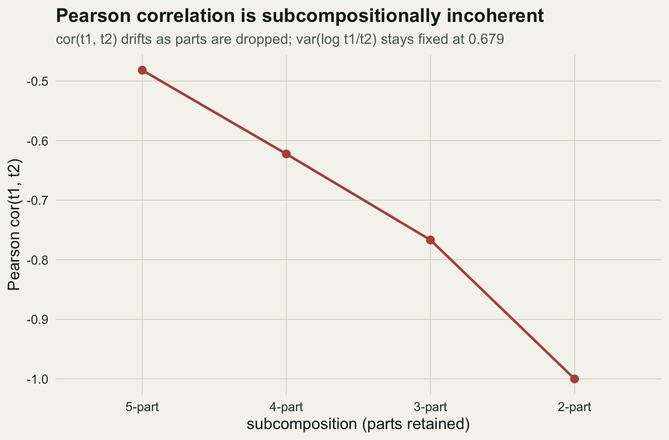
How often this misleads
To see that the negative bias is systematic and not a feature of one dataset, we can regenerate independent communities many times and record the mean pairwise correlation before and after closure.
set.seed(101)
B <- 2000L
mc <- replicate(B, {
  Xb <- sapply(seq_len(D), function(j) rlnorm(n, mu[j], sdlog[j]))
  Pb <- Xb / rowSums(Xb)
  c(abs = mean(cor(Xb)[upper.tri(diag(D))]),
    clo = mean(cor(Pb)[upper.tri(diag(D))]))
})
round(c(absolute_mean = mean(mc["abs",]),
        closed_mean   = mean(mc["clo",]),
        closed_lo = quantile(mc["clo",], .025),
        closed_hi = quantile(mc["clo",], .975)), 3)
absolute_mean closed_mean closed_lo.2.5% closed_hi.97.5%
0.000 -0.235 -0.240 -0.230 Across 2000 independent communities the mean correlation between absolute abundances sits at 0.000, as it should for independent parts, while the closed mean is -0.235 with a tight interval from -0.240 to -0.230. The negative correlation is not sampling noise that averages away; it is a fixed consequence of closure. A significance test on proportions from independent communities will report associations, because the null it tests is zero correlation and closure has moved the truth away from zero. The false positives are built into the data.
The honest limit
It is tempting to hope that some clever correction recovers the absolute correlations from the proportions. It cannot. Closure projects the data onto a lower-dimensional surface and discards the total. From proportions alone there is no way to know whether taxon one rose or every other taxon fell; both give the same composition. Compositional methods do not restore absolute abundances. What they offer is a set of quantities, ratios and their logarithms, that describe the parts relative to one another without inventing associations. That is a real restriction, and the final post in this series returns to it in full.
What comes next
The fix follows directly from the one quantity that behaved well here: the log-ratio. Taking logarithms of ratios moves the data off the constrained simplex and into ordinary space, where correlation, distance, and ordination mean what they usually mean. The next post builds the centred, additive, and isometric log-ratio transformations by hand and shows how they relate.
References
Aitchison J 1982 Journal of the Royal Statistical Society: Series B (Methodological) 44(2):139-160 (10.1111/j.2517-6161.1982.tb01195.x)
Aitchison J 1986 The Statistical Analysis of Compositional Data. Monographs on Statistics and Applied Probability. Chapman and Hall, London. ISBN 978-0-412-28060-3
Jackson DA 1997 Ecology 78(3):929-940 (10.1890/0012-9658(1997)078[0929:CDICET]2.0.CO;2)
Pearson K 1897 Proceedings of the Royal Society of London 60:489-498 (10.1098/rspl.1896.0076)
Gloor GB, Macklaim JM, Pawlowsky-Glahn V, Egozcue JJ 2017 Frontiers in Microbiology 8:2224 (10.3389/fmicb.2017.02224)