library(ggplot2)
clr <- function(x) { lx <- log(x); lx - mean(lx) }
ilr_basis <- function(D) {
  V <- matrix(0, D, D - 1)
  for (i in seq_len(D - 1)) { a <- sqrt(1 / (i * (i + 1))); b <- sqrt(i / (i + 1))
    V[1:i, i] <- a; V[i + 1, i] <- -b }
  V
}
te_ink <- "#16241d"; te_forest <- "#275139"; te_faint <- "#5d6b61"
te_paper <- "#f5f4ee"; te_line <- "#dad9ca"; te_red <- "#b5534e"
theme_te <- function(base = 12) theme_minimal(base_size = base) + theme(
  plot.background = element_rect(fill = te_paper, colour = NA),
  panel.background = element_rect(fill = te_paper, colour = NA),
  panel.grid.major = element_line(colour = te_line, linewidth = 0.3),
  panel.grid.minor = element_blank(),
  axis.text = element_text(colour = "#2c3a31"), axis.title = element_text(colour = te_ink),
  plot.title = element_text(colour = te_ink, face = "bold"),
  plot.subtitle = element_text(colour = te_faint, size = rel(0.9)), legend.position = "top")
theme_set(theme_te())Checking a compositional analysis
R
compositional data
ggplot2
reproducibility
ecology tutorial
Three diagnostics for a compositional result: does the verdict survive dropping a part, do the residuals behave, and what the unseen total can overturn.
The three previous posts built compositional data analysis from the ground up: closure distorts correlation and distance, log-ratios repair the geometry, and log-ratios localise a real change where naive proportion tests scatter false positives, once the zeros are dealt with. This closing post is about doubt. Given a compositional result, how do you check whether it holds, and how do you state its limit honestly? Three diagnostics answer that, and the last of them turns the central limitation of the whole approach into a single number a reader can argue with.
Setup
We reuse the two-group set-up, but with a sharper truth. Taxon one blooms, a threefold absolute increase; taxa two to six do not change in absolute abundance. The focal taxon is taxon two: truly flat, and the checks are about whether we can say so.
set.seed(7715)
D <- 6L; ng <- 70L; sdl <- rep(0.4, D)
mu <- c(3.2, 2.6, 2.4, 2.2, 2.0, 2.3)
sim <- function(m) sapply(1:D, function(j) rlnorm(ng, m[j], sdl[j]))
Xc <- sim(mu); mt <- mu; mt[1] <- mt[1] + log(3); Xt <- sim(mt)
Pc <- Xc / rowSums(Xc); Pt <- Xt / rowSums(Xt)
Check 1: does the verdict survive dropping a part?
The first diagnostic exploits subcompositional coherence directly. A conclusion that is really about two taxa should not change when an unrelated part is removed from the table. So run the analysis on the full composition, then drop the blooming taxon and re-close, and see whether the verdict for the focal taxon holds. For the naive proportion test it does not.
p2_full <- t.test(Pc[,2], Pt[,2])$p.value
subc <- Xc[,2:6] / rowSums(Xc[,2:6]); subt <- Xt[,2:6] / rowSums(Xt[,2:6])   # drop taxon 1
p2_sub <- t.test(subc[,1], subt[,1])$p.value                                  # taxon 2 is column 1 here
lr_full <- t.test(log(Xc[,2]/Xc[,3]), log(Xt[,2]/Xt[,3]))$p.value
lr_sub  <- t.test(log(subc[,1]/subc[,2]), log(subt[,1]/subt[,2]))$p.value
c(naive_full = p2_full, naive_drop_bloomer = p2_sub, coda_full = lr_full, coda_drop = lr_sub)
naive_full naive_drop_bloomer coda_full coda_drop
9.265552e-13 4.965387e-01 3.162609e-01 3.162609e-01 On the full composition the naive test declares taxon two strongly different, at \(9.3 \times 10^{-13}\). Remove the bloomer and re-close, and the same taxon is no longer significant, at 0.497. The verdict flipped on the presence of an unrelated part, which is a clear sign it was an artefact of closure rather than a fact about taxon two. The log-ratio verdict does not move: 0.316 on the full composition and 0.316 on the subcomposition, identical, because the ratio between two parts ignores everything else. When a naive and a coherent analysis disagree like this, the coherent one is the one to trust.
pv <- c(p2_full, p2_sub, lr_full, lr_sub)
dco <- data.frame(method = rep(c("naive proportion", "CoDA log-ratio"), each = 2),
                  comp = factor(rep(c("full 6-part", "drop the bloomer"), 2),
                                levels = c("full 6-part", "drop the bloomer")),
                  nl = -log10(pv))
p_coherence <- ggplot(dco, aes(comp, nl, fill = method)) +
  geom_col(position = position_dodge(0.7), width = 0.6) +
  geom_hline(yintercept = -log10(0.05), linetype = "dashed", colour = te_faint) +
  scale_fill_manual(values = c("naive proportion" = te_red, "CoDA log-ratio" = te_forest), name = NULL) +
  labs(title = "Does the verdict depend on which parts are in the table?",
       subtitle = "The focal taxon is truly unchanged; the naive verdict flips, the log-ratio verdict does not",
       x = NULL, y = "test for focal taxon  (-log10 p)")
p_coherence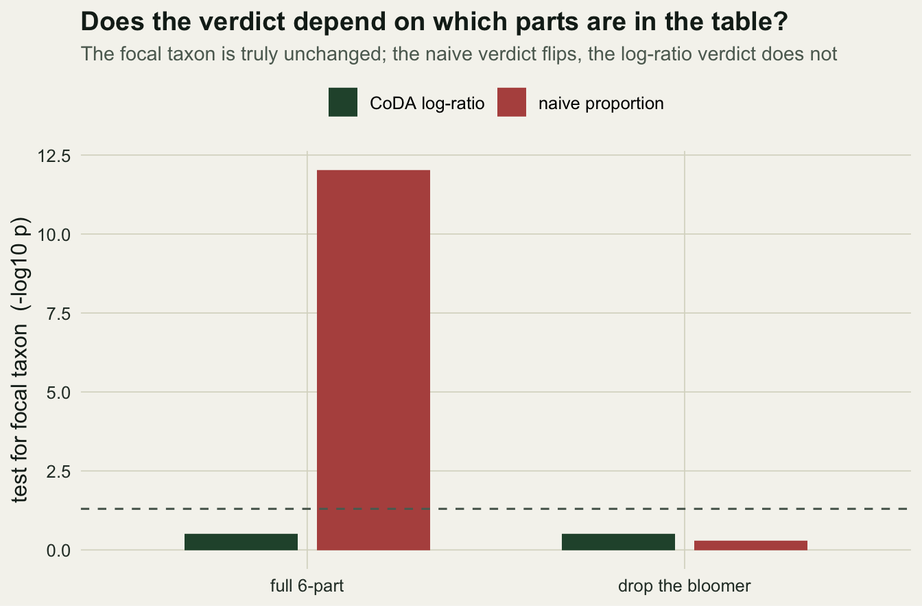
Check 2: do the model residuals behave?
The second diagnostic is the ordinary one, moved into the right coordinates. A model fitted in isometric log-ratio space produces residuals that should look like well-behaved multivariate noise if the model form is adequate. A per-coordinate normality test is a quick screen.
V <- ilr_basis(D)
Y <- rbind(Xc, Xt); ILR <- t(apply(Y, 1, clr)) %*% V
g <- factor(rep(c("c", "t"), each = ng))
res <- residuals(lm(ILR ~ g))
sh <- apply(res, 2, function(z) shapiro.test(z)$p.value)
c(min_shapiro_p = min(sh), coords = D - 1, all_pass = all(sh > 0.05))
min_shapiro_p coords all_pass
0.3155817 5.0000000 1.0000000 The smallest normality p-value across the 5 coordinates is 0.316, above the usual threshold, so the group model in ilr space is adequate for these data. It is worth being clear about what this checks and what it does not. It checks the form of the model, the distributional shape of the residuals. It says nothing about the reference frame, the assumption connecting relative to absolute change. A perfectly fitting compositional model can still mislead about absolute abundance, which is what the third check confronts.
Check 3: how far can an absolute claim be pushed?
This is the important one. Taxon two fell in relative terms, its proportion is lower in the treatment group, and it is tempting to report that taxon two decreased. But relative and absolute change differ by the change in the total, and the composition does not contain the total. Written on the log scale, the absolute change of taxon two equals its observed relative change plus the log of whatever the total did.
logFC_rel <- mean(log(Pt[,2])) - mean(log(Pc[,2]))       # observed relative change, < 0
r_star    <- exp(-logFC_rel)                              # total change at which absolute change is zero
true_total <- mean(rowSums(Xt)) / mean(rowSums(Xc))       # known here, unobservable from composition
c(relative_logFC = logFC_rel, tipping_total = r_star, true_total = true_total)
relative_logFC tipping_total true_total
-0.5727086 1.7730632 1.7636673 The observed relative change is -0.573, negative, so on proportions taxon two looks as though it went down. The tipping point is a total fold-change of 1.773: if the community total rose by less than that, taxon two really did decrease in absolute terms; if it rose by more, taxon two actually increased, and the relative drop was an illusion of everything else growing faster. In this simulation the true total change, which a field study would not measure, is 1.764. Read it against the tipping point just quoted: whichever side it falls on, and however far from the line it lands, the absolute direction of taxon two is decided by the unmeasured total, not by anything in the composition.
rs <- seq(1, 3.5, by = 0.05); dfr <- data.frame(r = rs, abs = logFC_rel + log(rs))
ggplot(dfr, aes(r, abs)) +
  annotate("rect", xmin = 1, xmax = r_star, ymin = -Inf, ymax = Inf, fill = te_red, alpha = 0.10) +
  annotate("rect", xmin = r_star, xmax = 3.5, ymin = -Inf, ymax = Inf, fill = te_forest, alpha = 0.10) +
  geom_hline(yintercept = 0, colour = te_faint) +
  geom_line(colour = te_ink, linewidth = 0.9) +
  geom_vline(xintercept = r_star, linetype = "dashed", colour = te_red) +
  geom_vline(xintercept = true_total, linetype = "dotted", colour = te_forest) +
  annotate("text", x = 1.05, y = max(dfr$abs) * 0.8, label = "taxon 2 absolutely down",
           hjust = 0, colour = te_red, size = 3.2) +
  annotate("text", x = 3.45, y = min(dfr$abs) * 0.8, label = "taxon 2 absolutely up",
           hjust = 1, colour = te_forest, size = 3.2) +
  labs(title = "The honest limit: the total is the missing information",
       subtitle = sprintf("Absolute change flips sign at r* = %.2f; the true hidden total change is %.2f", r_star, true_total),
       x = "assumed total-abundance fold-change (treatment / control)",
       y = "implied absolute log fold-change of taxon 2")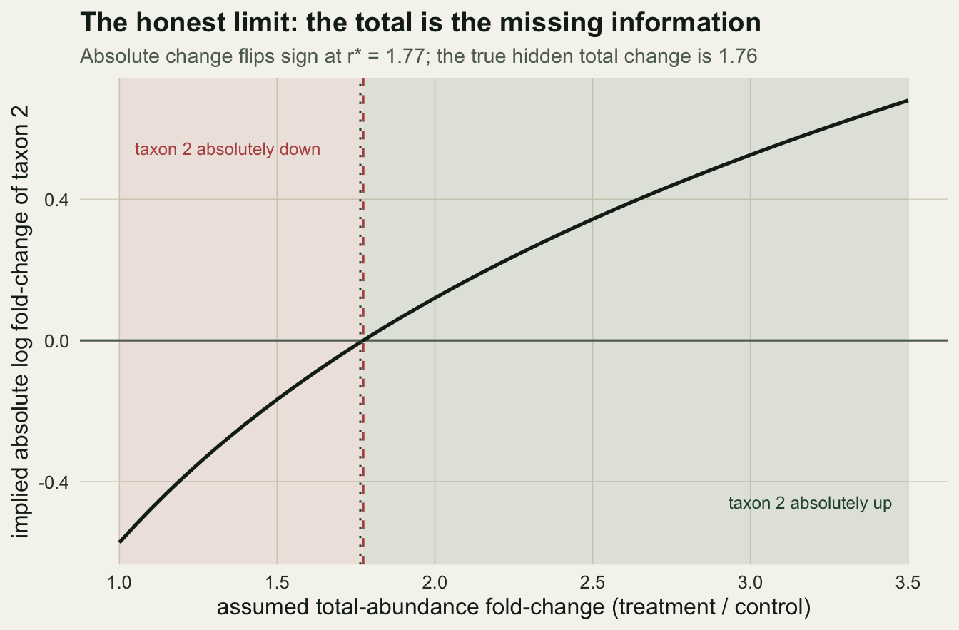
The honest limit, restated
The third check is the whole series in miniature. Compositional data carry relative information and nothing else. To make an absolute claim you must supply the total from outside the composition, whether from a spike-in, a measured density, or an assumption that some reference taxon held constant. That external input is untestable from the data, exactly as the mechanism behind a missing value is untestable, and exactly as the size of a measurement error is untestable. In each case the honest move is the same: do not hide the assumption, put a range on it, and report the point at which the conclusion turns over. Here that point is a total fold-change of 1.77. A reader can now judge for themselves whether the community total plausibly rose by more or less than that, which is a real scientific question, rather than being handed a relative change dressed up as an absolute one.
Closing the series
Four posts, one idea: the total that closure removes cannot be recovered, so proportions must be analysed as ratios, and any statement about absolute abundance needs information the composition does not hold. Log-ratios give a geometry where distance, ordination and testing work, zeros are handled by an explicit and reviewable imputation, and the reference-frame limit is stated as a tipping point instead of buried. That is the whole of what compositional data analysis asks for, and the whole of what it can honestly deliver.
References
Aitchison J 1986 The Statistical Analysis of Compositional Data, Chapman and Hall, ISBN 978-0-412-28060-3
Egozcue JJ, Pawlowsky-Glahn V 2005 Mathematical Geology 37(7):795-828 (10.1007/s11004-005-7381-9)
Morton JT, Marotz C, Washburne A, Silverman J, Zaramela LS, Edlund A, Zengler K, Knight R 2019 Nature Communications 10:2719 (10.1038/s41467-019-10656-5)
Lin H, Peddada SD 2020 Nature Communications 11:3514 (10.1038/s41467-020-17041-7)
Greenacre M 2018 Compositional Data Analysis in Practice, Chapman and Hall/CRC, ISBN 978-1-138-31661-4
Filzmoser P, Hron K, Templ M 2018 Applied Compositional Data Analysis: With Worked Examples in R, Springer, ISBN 978-3-319-96420-1