library(ggplot2)

te_pal <- list(forest = "#275139", green = "#2f8f63", sage = "#93a87f",
               clay = "#b5534e", gold = "#cda23f", line = "#dad9ca",
               ink = "#16241d", paper = "#f5f4ee")

theme_te <- function() {
  theme_minimal(base_size = 12) +
    theme(panel.grid.minor = element_blank(),
          panel.grid.major = element_line(colour = "#e7e6dc"),
          plot.background = element_rect(fill = "#f5f4ee", colour = NA),
          panel.background = element_rect(fill = "#f5f4ee", colour = NA),
          plot.title = element_text(face = "bold", colour = te_pal$ink),
          axis.title = element_text(colour = te_pal$ink),
          legend.position = "bottom")
}The abundance-occupancy relationship
R
macroecology
occupancy
ecology tutorial
ggplot2
Occupancy is a censored count, so much of the abundance-occupancy relationship is arithmetic: simulate it in R and measure what its scatter really records.
The atlas arrives with a map for every species and a table at the back. The table has two columns that everybody looks at: the number of grid squares a species was found in, and the mean count per square. Plot one against the other and the picture is always the same. The species that turn up everywhere are the ones that turn up in numbers where they turn up at all, and the species confined to a handful of squares are scarce inside those squares too. On log axes the cloud is close to a straight line, the correlation is high, and it holds for birds, beetles, plants and diatoms.
The interspecific abundance-occupancy relationship is among the most repeated patterns in macroecology, and it gets read as biology almost automatically. Species with broad niches can use more of the landscape and reach higher densities in it. Species with large populations send out enough dispersers to rescue local patches from extinction, so they occupy more of them. Both stories are plausible, both have literature behind them, and neither is what this post is about.
The objection is arithmetic. Occupancy is not an independent measurement of a species. It is the count data with everything above zero thrown away. Once a species has a mean density and a spatial distribution of individuals, its occupancy is fixed: there is nothing left to explain. A positive relationship between the two axes is therefore what you get from a model that contains no ecology at all, and the interesting question is not whether the relationship is there but whether anything is left in it after the arithmetic has been taken out.
So this post measures four things. What occupancy an identity says a species must have, given its density and how clumped it is. How strong an abundance-occupancy relationship a generating model with no biology in it produces. How much of the scatter around that relationship is a readout of spatial aggregation rather than of niche breadth. And what changing the grid or missing the species does to the slope everybody quotes.
The landscape is simulated, for the usual reason: a simulated assemblage comes with the generating parameters written down, so the mean density and the aggregation of every species are known rather than estimated, and any claim about what drives occupancy can be checked against what actually did. Mean density here is the generating parameter and not a sample statistic, which also means that nothing in the relationships below comes from sampling error shared between the two axes.
Two neighbouring posts cover the adjacent jobs and are not repeated here. Imperfect detection and occupancy fits the occupancy model that separates detection from presence, and zeta diversity across many sites treats the occupancy frequency distribution as a readout of turnover. This post stays on the ground between the two axes: what occupancy inherits from abundance, and what is left over.
Occupancy is a censored count
Take one species with mean density mu individuals per cell, and suppose the individuals fall independently, so the count in a cell is Poisson. The probability that a cell holds nothing is exp(-mu), so the expected occupancy is
\[\psi = 1 - e^{-\mu}\]
and that is the whole derivation. No parameter has been fitted and no biology has been assumed beyond the independence of individuals.
Individuals are not independent. They aggregate, and the standard one-parameter description of that is the negative binomial, whose aggregation parameter k runs from small values for a heavily clumped species up to infinity for a species with no clumping at all, where it reduces to the Poisson. Its probability of a zero is (1 + mu/k)^(-k), so
\[\psi = 1 - \left(1 + \frac{\mu}{k}\right)^{-k}\]
Both are identities, not models to be fitted, and both say the same thing: occupancy is a function of mean density and of one shape parameter, and nothing else enters. A simulator that disagrees with them is broken, so the first thing to do is check that this one does not.
occ_poisson <- function(mu) 1 - exp(-mu)
occ_nb <- function(mu, k) 1 - (1 + mu / k)^(-k)

set.seed(20260725)
n_cal <- 2e6
mu_cal <- c(0.1, 0.5, 2, 8)
k_cal <- c(1, 0.25)
lab <- c("Poisson", "NB k = 1", "NB k = 0.25")

cal <- NULL
for (j in seq_along(lab)) for (mu in mu_cal) {
  if (j == 1) {
    from_formula <- occ_poisson(mu)
    simulated <- mean(rpois(n_cal, mu) > 0)
  } else {
    kk <- k_cal[j - 1]
    from_formula <- occ_nb(mu, kk)
    simulated <- mean(rnbinom(n_cal, mu = mu, size = kk) > 0)
  }
  se <- sqrt(from_formula * (1 - from_formula) / n_cal)
  cal <- rbind(cal, c(mu = mu, formula = from_formula, simulated = simulated,
                      difference = simulated - from_formula,
                      z = (simulated - from_formula) / se))
}
rownames(cal) <- paste(rep(lab, each = length(mu_cal)), rep(mu_cal, 3))
print(round(cal, 5))
mu formula simulated difference z
Poisson 0.1 0.1 0.09516 0.09497 -0.00020 -0.94260
Poisson 0.5 0.5 0.39347 0.39316 -0.00031 -0.89261
Poisson 2 2.0 0.86466 0.86464 -0.00002 -0.08358
Poisson 8 8.0 0.99966 0.99965 -0.00001 -0.89099
NB k = 1 0.1 0.1 0.09091 0.09098 0.00007 0.35129
NB k = 1 0.5 0.5 0.33333 0.33323 -0.00011 -0.31900
NB k = 1 2 2.0 0.66667 0.66679 0.00012 0.36400
NB k = 1 8 8.0 0.88889 0.88894 0.00005 0.22550
NB k = 0.25 0.1 0.1 0.08068 0.08080 0.00013 0.65282
NB k = 0.25 0.5 0.5 0.24016 0.24065 0.00048 1.59796
NB k = 0.25 2 2.0 0.42265 0.42225 -0.00040 -1.15584
NB k = 0.25 8 8.0 0.58277 0.58313 0.00036 1.02859round(c(largest_absolute_difference = max(abs(cal[, "difference"])),
largest_difference_in_ses = max(abs(cal[, "z"])),
occupancy_at_density_1_poisson = occ_poisson(1),
occupancy_at_density_1_k_1 = occ_nb(1, 1),
occupancy_at_density_1_k_025 = occ_nb(1, 0.25)), 4) largest_absolute_difference largest_difference_in_ses
0.0005 1.5980
occupancy_at_density_1_poisson occupancy_at_density_1_k_1
0.6321 0.5000
occupancy_at_density_1_k_025
0.3313 Twelve combinations of density and aggregation, each one counted on a simulated landscape of two million cells. The largest disagreement between the count and the formula is 0.0005 in occupancy, which is 1.598 Monte Carlo standard errors, so the simulator and the identity are the same model. That check is worth the two minutes it takes to write. A previous post in this blog nearly published a reversed conclusion because the simulator and the closed form were quietly different things.
The numbers at the foot of the output are the point of the section. A species at a mean density of one individual per cell occupies 0.6321 of the landscape if its individuals are independent, 0.5 if they follow a negative binomial with k of 1, and 0.3313 if k is 0.25. Same density, same landscape, three different range sizes, and the only thing that changed was how the individuals are arranged.
grid_mu <- exp(seq(log(0.02), log(30), length.out = 300))
curve_df <- data.frame(
  mu = rep(grid_mu, 3),
  occ = c(occ_poisson(grid_mu), occ_nb(grid_mu, 1), occ_nb(grid_mu, 0.25)),
  model = factor(rep(lab, each = length(grid_mu)), levels = lab))
point_df <- data.frame(mu = cal[, "mu"], occ = cal[, "simulated"],
                       model = factor(rep(lab, each = length(mu_cal)),
                                      levels = lab))

ggplot(curve_df, aes(mu, occ, colour = model)) +
  geom_line(linewidth = 1.1) +
  geom_point(data = point_df, aes(shape = model), size = 2.8, stroke = 1.1) +
  scale_colour_manual(values = c(te_pal$forest, te_pal$gold, te_pal$clay),
                      name = NULL) +
  scale_shape_manual(values = c(16, 17, 15), name = NULL) +
  scale_x_log10(breaks = c(0.02, 0.1, 0.5, 2, 8, 30)) +
  scale_y_continuous(limits = c(0, 1), breaks = seq(0, 1, 0.2)) +
  labs(x = "Mean density (individuals per cell)", y = "Occupancy",
       title = "Occupancy is what is left of a count after censoring") +
  theme_te()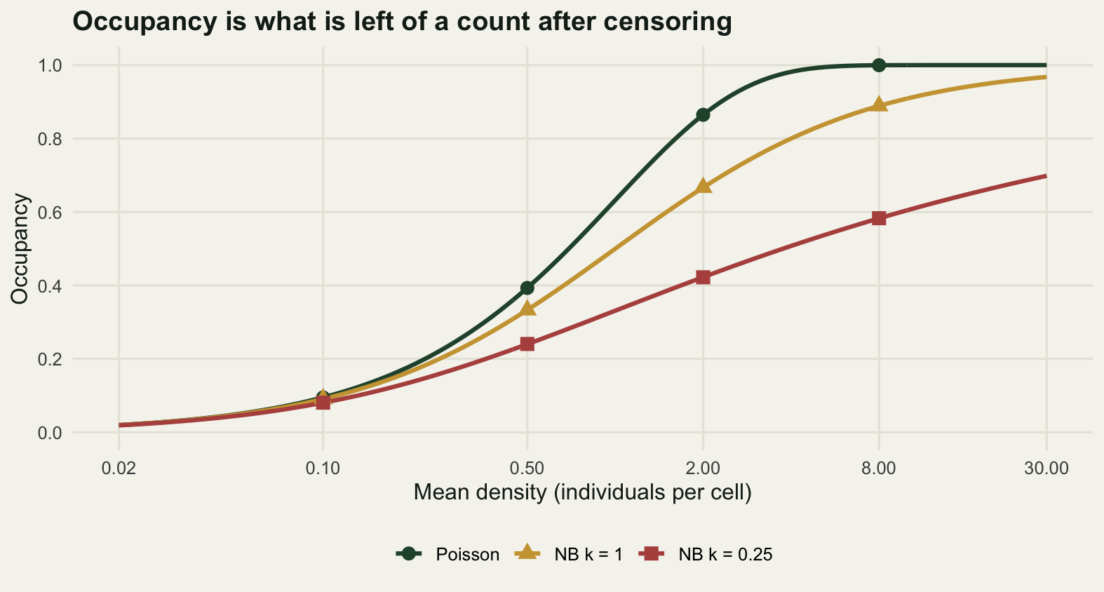
An assemblage with no biology in it
Now build an assemblage. A hundred and twenty species on a 128 by 128 grid of 16384 cells. Log mean densities are drawn from one normal distribution, which is the only species-level variation in the whole simulation. Every species gets the same aggregation parameter, k of 0.7. Nothing links occupancy to density except the censoring: there is no niche in the generator, no resource use, no dispersal, no metapopulation, no habitat.
set.seed(521)
n_side <- 128
n_cell <- n_side^2
n_sp <- 120
mu <- exp(rnorm(n_sp, log(0.7), 1.15))
k_one <- 0.7

cnt1 <- matrix(rnbinom(n_cell * n_sp, mu = rep(mu, each = n_cell), size = k_one),
               nrow = n_cell)
occ1 <- colMeans(cnt1 > 0)
aor1 <- lm(log(occ1) ~ log(mu))
slope_of <- function(f) as.numeric(coef(f)[2])
icept_of <- function(f) as.numeric(coef(f)[1])

round(c(grid_side = n_side, cells = n_cell, species = n_sp,
        aggregation_of_every_species = k_one,
        lowest_density = min(mu), highest_density = max(mu),
        lowest_occupancy = min(occ1), highest_occupancy = max(occ1)), 4)
grid_side cells
128.0000 16384.0000
species aggregation_of_every_species
120.0000 0.7000
lowest_density highest_density
0.0150 6.5440
lowest_occupancy highest_occupancy
0.0135 0.8044 round(c(log_log_slope = slope_of(aor1), log_log_intercept = icept_of(aor1),
log_log_correlation = cor(log(mu), log(occ1)),
log_log_r_squared = summary(aor1)$r.squared,
logit_slope = slope_of(lm(qlogis(occ1) ~ log(mu))),
logit_correlation = cor(log(mu), qlogis(occ1)),
largest_gap_from_the_identity = max(abs(occ1 - occ_nb(mu, k_one)))), 4) log_log_slope log_log_intercept
0.6304 -0.8719
log_log_correlation log_log_r_squared
0.9744 0.9495
logit_slope logit_correlation
0.9264 0.9990
largest_gap_from_the_identity
0.0095 The mean densities span 0.0150 to 6.5440 individuals per cell and the occupancies span 0.0135 to 0.8044, so the assemblage spans the range an atlas spans, from species with a toehold in the grid to species in four squares out of five. The relationship across those 120 species has a log-log slope of 0.6304 and a correlation of 0.9744. On the logit scale, which is the other common way to fit it, the slope is 0.9264 and the correlation is 0.9990.
That is a stronger relationship than most published ones, from a generating model in which the species differ in exactly one thing. It is worth saying plainly what it means. If a paper reports a positive abundance-occupancy relationship with a correlation of 0.9744 and offers niche breadth as the explanation, the pattern it reports is fully reproduced by a model containing no niches. The pattern is not evidence for the explanation, because it is not evidence against anything.
The other number in the output says why the relationship is so tight. Every simulated occupancy is within 0.0095 of the value the identity predicts from that species’ density and k. There is no scatter to speak of, because in this assemblage there is nothing for the scatter to be made of: two species with the same density have the same occupancy, up to the sampling variation of 16384 cells.
line_mu <- exp(seq(log(min(mu)), log(max(mu)), length.out = 300))
aor_lines <- data.frame(
  mu = rep(line_mu, 2),
  occ = c(occ_nb(line_mu, k_one),
          exp(icept_of(aor1) + slope_of(aor1) * log(line_mu))),
  series = factor(rep(c("Censoring identity at k = 0.7", "Fitted power law"),
                      each = length(line_mu)),
                  levels = c("Censoring identity at k = 0.7",
                             "Fitted power law")))

ggplot(data.frame(mu = mu, occ = occ1), aes(mu, occ)) +
  geom_point(colour = te_pal$sage, size = 2.4, alpha = 0.9) +
  geom_line(data = aor_lines, aes(colour = series, linetype = series),
            linewidth = 1.0) +
  scale_colour_manual(values = c(te_pal$forest, te_pal$clay), name = NULL) +
  scale_linetype_manual(values = c(1, 2), name = NULL) +
  scale_x_log10() +
  scale_y_log10() +
  labs(x = "Mean density (individuals per cell)", y = "Occupancy",
       title = "A tight relationship out of a model with no ecology in it") +
  theme_te()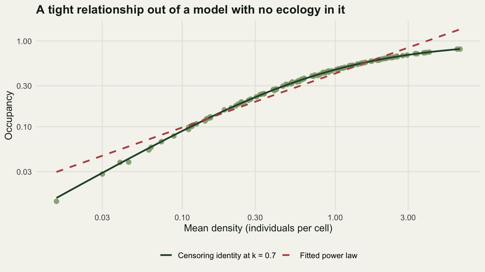
The figure carries a second point that the correlation hides. The identity is a curve and the fitted power law is a straight line, so the fit is wrong in a systematic way at both ends even though its R squared is 0.9495. Five per cent of unexplained variance, in an assemblage with no biological variation whatsoever, is not noise: it is the wrong functional form. That matters in the next section, where residuals from the straight line are asked to carry a meaning.
The scatter is a map of aggregation
Real assemblages do not have one value of k. Some species are heavily clumped and some are spread out, and the difference is a property worth having: it is the thing the censoring identity says should move occupancy at a fixed density. So draw k from a distribution as well, independently of density, and repeat.
set.seed(913)
kv <- exp(rnorm(n_sp, log(0.7), 0.6))
cnt2 <- matrix(rnbinom(n_cell * n_sp, mu = rep(mu, each = n_cell),
                       size = rep(kv, each = n_cell)), nrow = n_cell)
occ2 <- colMeans(cnt2 > 0)
aor2 <- lm(log(occ2) ~ log(mu))
res2 <- resid(aor2)

k_mid <- median(kv)
dev_obs <- log(occ2) - log(occ_nb(mu, k_mid))
dev_pred <- log(occ_nb(mu, kv)) - log(occ_nb(mu, k_mid))
crude <- lm(res2 ~ log(kv))
against_identity <- lm(dev_obs ~ dev_pred)

round(c(lowest_k = min(kv), median_k = k_mid, highest_k = max(kv),
        correlation_of_density_and_k = cor(log(mu), log(kv)),
        log_log_slope = slope_of(aor2),
        r_squared_of_the_fit = summary(aor2)$r.squared,
        residual_sd = sd(res2),
        residual_on_log_k_r_squared = summary(crude)$r.squared,
        deviation_on_prediction_r_squared = summary(against_identity)$r.squared,
        deviation_on_prediction_slope = slope_of(against_identity),
        deviation_on_prediction_icept = icept_of(against_identity),
        share_above_the_median_k_identity = mean(occ2 > occ_nb(mu, k_mid)),
        share_above_the_highest_k_identity = mean(occ2 > occ_nb(mu, max(kv)))), 4)
lowest_k median_k
0.1724 0.7242
highest_k correlation_of_density_and_k
2.6241 -0.0264
log_log_slope r_squared_of_the_fit
0.6095 0.9176
residual_sd residual_on_log_k_r_squared
0.2211 0.3978
deviation_on_prediction_r_squared deviation_on_prediction_slope
0.9874 1.0031
deviation_on_prediction_icept share_above_the_median_k_identity
0.0019 0.5250
share_above_the_highest_k_identity
0.0333 Aggregation now ranges from 0.1724 to 2.6241 across the assemblage and is uncorrelated with density by construction, at -0.0264. The relationship survives: slope 0.6095, R squared 0.9176. What changed is that there is now real scatter around it, with a residual standard deviation of 0.2211 on the log scale.
An ecologist looking at that scatter has a decision to make about what it means. The usual reading is that the residual is the biology: species sitting above the line occupy more than their abundance warrants, so they must be good dispersers or habitat generalists, and species below it must be specialists. Regress the residual on the aggregation parameter and 39.78 per cent of it goes at once: that much of the scatter around the fitted line is accounted for by how clumped each species is, and by nothing else.
The rest of that scatter is not biology either. It is the curvature from the previous section: the straight line is the wrong shape, so its residuals contain a smooth function of density on top of everything else. Take that out by comparing like with like. Each species has a deviation from the identity curve evaluated at the assemblage median k of 0.7242, and the identity, given that species’ own k, predicts exactly what that deviation should be. Regressing the observed deviation on the predicted one gives a slope of 1.0031, an intercept of 0.0019 and an R squared of 0.9874.
So the answer is that essentially all of it is aggregation. The scatter about an abundance-occupancy relationship is, in this assemblage, a measurement of how clumped the species are, dressed up as a measurement of how they use the landscape. Whatever niche breadth contributes has to live in what is left once that 0.9874 has been taken out, and in a real dataset it is competing with sampling error as well.
The size of the effect is easier to feel with two species than with a regression. Take the median density in the assemblage and give it to a species at the fifth percentile of aggregation and to one at the ninety-fifth.
set.seed(77)
mu_fixed <- median(mu)
k_low <- as.numeric(quantile(kv, 0.05))
k_high <- as.numeric(quantile(kv, 0.95))

round(c(density_of_both = mu_fixed,
        aggregation_clumped = k_low, aggregation_even = k_high,
        occupancy_clumped = mean(rnbinom(n_cell, mu = mu_fixed,
                                         size = k_low) > 0),
        occupancy_even = mean(rnbinom(n_cell, mu = mu_fixed,
                                      size = k_high) > 0),
        identity_clumped = occ_nb(mu_fixed, k_low),
        identity_even = occ_nb(mu_fixed, k_high),
        ratio_of_the_identities = occ_nb(mu_fixed, k_high) /
          occ_nb(mu_fixed, k_low)), 4)
density_of_both aggregation_clumped aggregation_even
0.7129 0.2678 1.5915
occupancy_clumped occupancy_even identity_clumped
0.2925 0.4438 0.2936
identity_even ratio_of_the_identities
0.4451 1.5160 Two species at a density of 0.7129 individuals per cell. The clumped one, k of 0.2678, occupies 0.2925 of the landscape. The even one, k of 1.5915, occupies 0.4438, and the identity puts the ratio at 1.5160. On an atlas map that is the difference between a species that looks locally distributed and a species that looks widespread, and the two have identical population sizes. Both counted occupancies sit where the identity puts them: 0.2925 against 0.2936, and 0.4438 against 0.4451.
k_show <- c(min(kv), median(kv), max(kv))
band_df <- data.frame(
  mu = rep(line_mu, 3),
  occ = c(occ_nb(line_mu, k_show[1]), occ_nb(line_mu, k_show[2]),
          occ_nb(line_mu, k_show[3])),
  k = rep(k_show, each = length(line_mu)),
  grp = factor(rep(seq_along(k_show), each = length(line_mu))))

# the top two curves sit within a few pixels of each other, so each one says
# which k it is rather than leaving the colour bar to be read backwards
band_lab <- data.frame(mu = max(line_mu) * 1.07,
                       occ = occ_nb(max(line_mu), k_show),
                       txt = sprintf("k = %.2f", k_show),
                       vj = c(0.5, 1.2, -0.3))

ggplot(data.frame(mu = mu, occ = occ2, k = kv), aes(mu, occ, colour = k)) +
  geom_line(data = band_df, aes(group = grp), linewidth = 1.0) +
  geom_point(size = 2.6) +
  geom_text(data = band_lab, aes(mu, occ, label = txt, vjust = vj),
            inherit.aes = FALSE, hjust = 0, size = 3.1, colour = te_pal$ink) +
  scale_colour_gradient(low = te_pal$gold, high = te_pal$forest,
                        trans = "log10", breaks = c(0.2, 0.5, 1, 2),
                        name = "Aggregation k (log scale)") +
  scale_x_log10() +
  scale_y_log10() +
  expand_limits(x = max(line_mu) * 2.1) +
  guides(colour = guide_colourbar(barwidth = 12, barheight = 0.6)) +
  labs(x = "Mean density (individuals per cell)", y = "Occupancy",
       title = "The scatter sorts by aggregation, not by chance") +
  theme_te()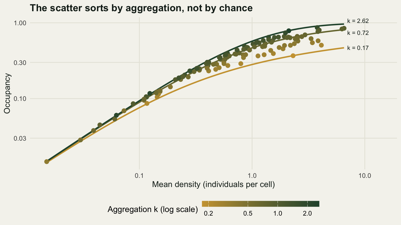
Occupancy is a property of the grid
Nothing so far has mentioned the size of a cell, and that is the next problem, because occupancy is not a property of a species. It is a property of a species and a grid. Change the grid and every number in the table at the back of the atlas changes, including the slope.
Aggregating the same landscape into blocks of 2 by 2, 4 by 4 and 8 by 8 cells answers it directly. The individuals do not move: only the lines drawn round them change. A second landscape is built alongside for comparison, with the same species, the same mean densities and the same aggregation, but with the clumping arranged spatially: a gamma multiplier shared by all the cells in a patch of 8 by 8, and Poisson counts within cells. A Poisson count with a gamma mean is a negative binomial, so the two landscapes have the same count distribution in a cell and the same expected occupancy at the finest grain. What differs is where the empty cells are.
row_of <- rep(seq_len(n_side), times = n_side)
col_of <- rep(seq_len(n_side), each = n_side)
block_of <- function(g) ((row_of - 1) %/% g) * (n_side / g) +
  ((col_of - 1) %/% g) + 1
aggregate_to <- function(m, g) if (g == 1) m else rowsum(m, block_of(g))

set.seed(3311)
patch <- block_of(8)
gam <- matrix(rgamma(n_sp * max(patch), shape = k_one, scale = 1 / k_one),
              nrow = max(patch))
cnt_patchy <- matrix(rpois(n_cell * n_sp, gam[patch, ] * rep(mu, each = n_cell)),
                     nrow = n_cell)
occ_patchy1 <- colMeans(cnt_patchy > 0)

grains <- c(1, 2, 4, 8)
grain_tab <- NULL
for (g in grains) {
  o_ind <- colMeans(aggregate_to(cnt1, g) > 0)
  o_pat <- colMeans(aggregate_to(cnt_patchy, g) > 0)
  grain_tab <- rbind(grain_tab, c(
    block_width = g, blocks = n_cell / g^2,
    slope_independent = slope_of(lm(log(o_ind) ~ log(mu))),
    slope_patchy = slope_of(lm(log(o_pat) ~ log(mu))),
    mean_occ_independent = mean(o_ind), mean_occ_patchy = mean(o_pat),
    saturated_independent = sum(o_ind > 0.999),
    saturated_patchy = sum(o_pat > 0.999),
    spearman_independent = cor(occ1, o_ind, method = "spearman"),
    spearman_patchy = cor(occ_patchy1, o_pat, method = "spearman"),
    gap_from_the_independence_rule =
      max(abs(o_ind - (1 - (1 - occ_nb(mu, k_one))^(g^2))))))
}
print(round(grain_tab, 4))
block_width blocks slope_independent slope_patchy mean_occ_independent
[1,] 1 16384 0.6304 0.6268 0.3906
[2,] 2 4096 0.3813 0.3774 0.7641
[3,] 4 1024 0.1190 0.1824 0.9485
[4,] 8 256 0.0169 0.0740 0.9938
mean_occ_patchy saturated_independent saturated_patchy
[1,] 0.3915 0 0
[2,] 0.6316 0 0
[3,] 0.8135 69 0
[4,] 0.9176 113 0
spearman_independent spearman_patchy gap_from_the_independence_rule
[1,] 1.0000 1.0000 0.0095
[2,] 0.9994 0.9977 0.0197
[3,] 0.9193 0.9846 0.0347
[4,] 0.4062 0.9355 0.0193round(c(mean_occupancy_independent = mean(occ1),
mean_occupancy_patchy = mean(occ_patchy1),
largest_gap_between_landscapes = max(abs(occ1 - occ_patchy1)),
correlation_between_landscapes = cor(occ1, occ_patchy1)), 4) mean_occupancy_independent mean_occupancy_patchy
0.3906 0.3915
largest_gap_between_landscapes correlation_between_landscapes
0.0416 0.9977 The two landscapes start in the same place, as they were built to: mean occupancy 0.3906 against 0.3915, correlated at 0.9977 across species, no species differing by more than 0.0416. At the finest grain they are the same assemblage by every measure an atlas would report.
Three steps of coarsening take them apart. In the landscape with independent cells the slope falls from 0.6304 to 0.3813 to 0.1190 to 0.0169, and mean occupancy climbs from 0.3906 to 0.9938. By the coarsest grain 113 of the 120 species are in every block, so there is no relationship left to have a slope: everything is ubiquitous and the atlas has become a list. In the patchy landscape the same coarsening leaves the slope at 0.0740 and mean occupancy at 0.9176, with no species saturating at all, because a species whose empty cells are next to each other keeps empty blocks for longer.
The independent case has an exact answer, which is worth having because it is the fastest possible saturation. If cells are independent, a block of m cells is empty when all m are, so occupancy at block size m is 1 - (1 - psi)^m. Across all four grains the counted occupancy never departs from that rule by more than 0.0347. Coarsening is not mysterious. It is the same censoring applied to a bigger container.
The two Spearman columns are the practical part. The rank order of species survives coarsening far better than their occupancy values do: the Spearman correlation with the finest grain stays at 0.9994 and 0.9193 through the first two steps in the independent landscape, and 0.9977 and 0.9846 in the patchy one. It collapses to 0.4062 at the coarsest grain in the independent landscape, but that is saturation rather than reordering, because 113 tied species cannot be ranked. In the patchy landscape, where nothing saturates, the rank correlation is still 0.9355 after the cell has grown from one square to a block of 8 by 8. So an occupancy is comparable across studies only as a rank, and only while there is something left to rank.
What imperfect detection does, and does not, do
The last thing between the atlas and the truth is that a species present in a square is not always recorded there. Two ways of writing that down look similar and behave completely differently.
The first is the standard occupancy model’s detection process: each visit to an occupied cell finds the species with probability p, independent of how many individuals are in it. With three visits at p of 0.4, an occupied cell is recorded with probability 0.7840.
The second lets detection depend on abundance, which is what happens in the field: a cell holding one individual is harder to work than a cell holding twenty. Give each individual a probability r of 0.15 of being detected on a visit, so a cell holding N individuals is recorded across three visits with probability 1 - (1 - r)^(3N). That is 0.3859 for a single individual and 0.9126 for five.
I expected both to steepen the relationship, on the reasoning that rare species are missed most. Only one of them does.
p_visit <- 0.4
n_visit <- 3
r_ind <- 0.15
set.seed(8080)

det_tab <- NULL
keep_flat <- keep_abund <- NULL
for (g in grains) {
  a <- aggregate_to(cnt1, g)
  nb <- nrow(a)
  o_true <- colMeans(a > 0)
  o_flat <- colMeans((a > 0) & (matrix(runif(nb * n_sp), nb) <
                                  1 - (1 - p_visit)^n_visit))
  o_abund <- colMeans(matrix(runif(nb * n_sp), nb) <
                        1 - (1 - r_ind)^(a * n_visit))
  if (g == 1) {
    keep_flat <- o_flat / o_true
    keep_abund <- o_abund / o_true
  }
  det_tab <- rbind(det_tab, c(
    block_width = g,
    slope_true = slope_of(lm(log(o_true) ~ log(mu))),
    slope_flat = slope_of(lm(log(o_flat) ~ log(mu))),
    slope_abundance = slope_of(lm(log(o_abund) ~ log(mu))),
    icept_true = icept_of(lm(log(o_true) ~ log(mu))),
    icept_flat = icept_of(lm(log(o_flat) ~ log(mu))),
    occupancy_kept_flat = mean(o_flat / o_true),
    occupancy_kept_abundance = mean(o_abund / o_true)))
}
print(round(det_tab, 4))
block_width slope_true slope_flat slope_abundance icept_true icept_flat
[1,] 1 0.6304 0.6311 0.7795 -0.8719 -1.1148
[2,] 2 0.3813 0.3814 0.5958 -0.1873 -0.4308
[3,] 4 0.1190 0.1186 0.2783 -0.0152 -0.2592
[4,] 8 0.0169 0.0158 0.0697 0.0004 -0.2467
occupancy_kept_flat occupancy_kept_abundance
[1,] 0.7841 0.5511
[2,] 0.7838 0.7012
[3,] 0.7837 0.8901
[4,] 0.7818 0.9760round(c(visits = n_visit, detection_per_visit_flat = p_visit,
detection_per_individual = r_ind,
cell_recorded_if_occupied_flat = 1 - (1 - p_visit)^n_visit,
cell_recorded_if_it_holds_one = 1 - (1 - r_ind)^n_visit,
cell_recorded_if_it_holds_five = 1 - (1 - r_ind)^(5 * n_visit),
slope_ratio_flat = as.numeric(det_tab[1, 3] / det_tab[1, 2]),
slope_ratio_abundance = as.numeric(det_tab[1, 4] / det_tab[1, 2]),
intercept_shift_flat = as.numeric(det_tab[1, 6] - det_tab[1, 5]),
intercept_shift_expected = log(1 - (1 - p_visit)^n_visit),
occupancy_kept_rarest = as.numeric(keep_abund[which.min(mu)]),
occupancy_kept_commonest = as.numeric(keep_abund[which.max(mu)])), 4) visits detection_per_visit_flat
3.0000 0.4000
detection_per_individual cell_recorded_if_occupied_flat
0.1500 0.7840
cell_recorded_if_it_holds_one cell_recorded_if_it_holds_five
0.3859 0.9126
slope_ratio_flat slope_ratio_abundance
1.0011 1.2366
intercept_shift_flat intercept_shift_expected
-0.2429 -0.2433
occupancy_kept_rarest occupancy_kept_commonest
0.4661 0.8226 Detection that ignores abundance does not touch the slope. It multiplies every species’ occupancy by the same 0.7840, and multiplying by a constant is an additive shift on the log scale, so the slope ratio is 1.0011 and the intercept moves by -0.2429 against an expected -0.2433. The relationship is displaced downwards and is otherwise exactly the relationship you had. If detection really were flat across species, an unadjusted atlas would give the correct abundance-occupancy slope from biased occupancies, which is a strange and useful fact.
Detection that depends on abundance steepens it, by a factor of 1.2366 at the finest grain, from 0.6304 to 0.7795. The mechanism is in the last two numbers. The commonest species keeps 0.8226 of its occupancy and the rarest keeps 0.4661, because the cells an uncommon species occupies mostly hold one individual, and a cell holding one individual is recorded with probability 0.3859. The bias is not in the occupancy of a species, it is in the difference between species, and it is the largest where the pattern is read most confidently: at the bottom left of the plot.
The practical version: a survey with fixed effort per square makes the abundance-occupancy relationship look steeper and tighter than it is, and the steepening is worse the shorter the visit list. This is exactly the heterogeneity that the Royle-Nichols model was built for, and abundance from repeat detections fits it rather than assuming it away.
ser <- c("Independent cells", "Patchy landscape",
         "Constant detection per visit", "Detection rises with abundance")
sweep_df <- rbind(
  data.frame(g = grains, slope = grain_tab[, "slope_independent"],
             series = ser[1], panel = "Spatial arrangement"),
  data.frame(g = grains, slope = grain_tab[, "slope_patchy"],
             series = ser[2], panel = "Spatial arrangement"),
  data.frame(g = grains, slope = det_tab[, "slope_true"],
             series = ser[1], panel = "Detection"),
  data.frame(g = grains, slope = det_tab[, "slope_flat"],
             series = ser[3], panel = "Detection"),
  data.frame(g = grains, slope = det_tab[, "slope_abundance"],
             series = ser[4], panel = "Detection"))
sweep_df$series <- factor(sweep_df$series, levels = ser)
sweep_df$panel <- factor(sweep_df$panel,
                         levels = c("Spatial arrangement", "Detection"))

ggplot(sweep_df, aes(g, slope, colour = series, shape = series,
                     linetype = series, linewidth = series)) +
  geom_line() +
  geom_point(size = 2.9) +
  facet_wrap(~panel) +
  scale_colour_manual(values = c(te_pal$forest, te_pal$sage, te_pal$gold,
                                 te_pal$clay), name = NULL) +
  scale_shape_manual(values = c(16, 17, 15, 18), name = NULL) +
  scale_linetype_manual(values = c(1, 1, 2, 1), name = NULL) +
  scale_linewidth_manual(values = c(1.6, 1.0, 0.9, 1.0), name = NULL) +
  scale_x_continuous(transform = "log2", breaks = grains) +
  scale_y_continuous(limits = c(0, 0.85)) +
  guides(colour = guide_legend(nrow = 2), shape = guide_legend(nrow = 2),
         linetype = guide_legend(nrow = 2),
         linewidth = guide_legend(nrow = 2)) +
  labs(x = "Block width (cells)", y = "Fitted log-log slope",
       title = "Grid and effort move the slope more than biology needs to") +
  theme_te() +
  theme(strip.text = element_text(colour = te_pal$ink, face = "bold", size = 9),
        plot.margin = margin(6, 14, 6, 6))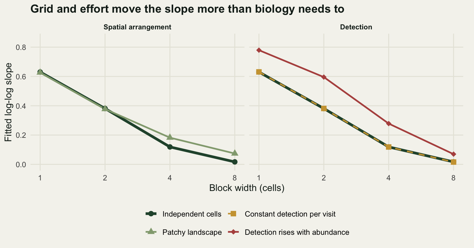
The honest limit: what occurrence data cannot settle
Everything above shows that censoring is sufficient to produce the pattern. It does not show that censoring is what produced any particular one, and it cannot, because the alternative explanations predict the same picture. Here is that degeneracy as a measurement rather than as a caveat.
Build a second assemblage on a different mechanism. Each species has a niche breadth. Broad-niched species find a larger fraction of the landscape suitable and reach higher densities where they occur, which is the resource use hypothesis in its simplest form. Inside its suitable habitat every species has the same aggregation, k of 0.7, so there is no variation in clumping to explain anything. Then choose the five free parameters so that this assemblage reproduces the first one’s fitted line, its residual spread and its distribution of mean densities, and simulate it.
target <- c(icept_of(aor2), slope_of(aor2), sd(res2), mean(log(mu)), sd(log(mu)))
set.seed(404)
breadth <- rnorm(n_sp)
noise_d <- rnorm(n_sp)
noise_s <- rnorm(n_sp)

brown <- function(p) {
  s <- plogis(p[1] + exp(p[2]) * breadth + p[5] * noise_s)
  d <- exp(p[3] + 0.3 * exp(p[2]) * breadth + p[4] * noise_d)
  list(suitable = s, density = d, mu = s * d,
       occ = s * (1 - (1 + d / k_one)^(-k_one)))
}
cost <- function(p) {
  z <- brown(p)
  if (any(!is.finite(log(z$occ)))) return(1e8)
  f <- lm(log(z$occ) ~ log(z$mu))
  sum((c(icept_of(f), slope_of(f), sd(resid(f)), mean(log(z$mu)),
         sd(log(z$mu))) - target)^2 * c(20, 20, 200, 20, 20))
}
op <- optim(c(0, 0, 0, 0.2, 0.2), cost,
            control = list(maxit = 9000, reltol = 1e-13))
op <- optim(op$par, cost, control = list(maxit = 9000, reltol = 1e-13))
z <- brown(op$par)

set.seed(2626)
cntB <- matrix(0L, n_cell, n_sp)
for (i in seq_len(n_sp)) {
  ns <- round(z$suitable[i] * n_cell)
  cntB[sample.int(n_cell, ns), i] <- rnbinom(ns, mu = z$density[i],
                                             size = k_one)
}
occB <- colMeans(cntB > 0)
aorB <- lm(log(occB) ~ log(z$mu))

round(c(suitable_fraction_lowest = min(z$suitable),
        suitable_fraction_highest = max(z$suitable),
        density_where_suitable_lowest = min(z$density),
        density_where_suitable_highest = max(z$density),
        slope_censoring = slope_of(aor2), slope_niche = slope_of(aorB),
        icept_censoring = icept_of(aor2), icept_niche = icept_of(aorB),
        r_squared_censoring = summary(aor2)$r.squared,
        r_squared_niche = summary(aorB)$r.squared,
        residual_sd_censoring = sd(res2), residual_sd_niche = sd(resid(aorB))), 4)
suitable_fraction_lowest suitable_fraction_highest
0.0333 1.0000
density_where_suitable_lowest density_where_suitable_highest
0.0180 14.7415
slope_censoring slope_niche
0.6095 0.6125
icept_censoring icept_niche
-0.9022 -0.9031
r_squared_censoring r_squared_niche
0.9176 0.9162
residual_sd_censoring residual_sd_niche
0.2211 0.2242 pool <- data.frame(log_occ = c(log(occ2), log(occB)),
log_mu = c(log(mu), log(z$mu)),
model = factor(rep(c("censoring", "niche"), each = n_sp),
levels = c("censoring", "niche")))
both <- lm(log_occ ~ log_mu * model, data = pool)
ks <- ks.test(res2, resid(aorB))
skew <- function(x) mean((x - mean(x))^3) / sd(x)^3
round(c(model_shift_p = summary(both)$coefficients[3, 4],
interaction_p = summary(both)$coefficients[4, 4],
ks_statistic = as.numeric(ks$statistic), ks_p_value = ks$p.value,
residual_skew_censoring = skew(res2),
residual_skew_niche = skew(resid(aorB))), 4) model_shift_p interaction_p ks_statistic
0.9767 0.9031 0.2417
ks_p_value residual_skew_censoring residual_skew_niche
0.0018 -1.0078 -2.5294 The two assemblages come from mechanisms with nothing in common. In one, occupancy is censored abundance and the scatter is aggregation. In the other, every species is equally aggregated and the pattern comes from how much of the landscape suits it. Their abundance-occupancy relationships are the same relationship: slope 0.6095 against 0.6125, intercept -0.9022 against -0.9031, R squared 0.9176 against 0.9162. Fit them together with an interaction and the difference in intercept has a p-value of 0.9767 and the difference in slope 0.9031.
Everything a paper reports about an abundance-occupancy relationship is in that list, and none of it separates the two. What does separate them is the shape of the scatter: the residuals are more left-skewed under the niche mechanism, -2.5294 against -1.0078, and a two-sample test on them gives a statistic of 0.2417 with a p-value of 0.0018. That test needed both assemblages side by side. A real study has one, so the comparison is not available to it, and the residual skew of a single sample of 120 species is not something anyone would bet a mechanism on.
The evidence that would separate them is not in the occurrence data at all. Two kinds would do it. Aggregation measured directly, within occupied habitat, so that the identity’s prediction can be tested rather than assumed: the censoring account says the residual is a function of k and the niche account says k is constant. Or density estimated independently at fixed occupancy, from counts rather than from presences, so that the two axes stop being computed from the same numbers. This post supplies neither. It measures the size of the arithmetic component and shows it is large enough to account for the whole pattern, which is a claim about what the data cannot rule out and not about what is true in any particular assemblage.
Three further limits are worth stating. The aggregation used throughout is a single negative binomial parameter, which is a summary of clumping and not a description of it: two very different spatial patterns can share a k, and the patchy landscape in the grain section is one demonstration of that. The species here are independent of one another, so nothing in this post says anything about how competition or shared habitat moves the pattern. And the grain sweep coarsens a fixed landscape rather than surveying at a coarser grain, so it isolates the effect of the container from the effect of the effort, which in a real atlas arrive together.
Where to go next
The most direct follow-on is range size distributions, which asks what the distribution of the occupancy axis looks like on its own and where its shape comes from. The other half of that pair is species abundance distributions, the distribution of the density axis, which is the input this post censors. If you want to test whether a macroecological pattern of this kind is doing any work at all, checking a macroecological pattern sets out the null models to run before believing one.
For the modelling rather than the pattern, imperfect detection and occupancy is the estimator that removes the flat part of the detection bias measured above, and N-mixture models go after the abundance behind the detections, which is what you need if you want the density axis and the occupancy axis to come from different data. For the count model that produced every landscape here, GLMs for count data covers where the negative binomial and its aggregation parameter come from, and species-area relationships is the same grain problem asked of richness rather than of one species at a time.
References
Brown JH 1984 The American Naturalist 124(2):255-279 (10.1086/284267)
Hanski I 1982 Oikos 38(2):210 (10.2307/3544021)
Wright DH 1991 Journal of Biogeography 18(4):463 (10.2307/2845487)
He F, Gaston KJ 2000 The American Naturalist 156(5):553-559 (10.1086/303403)
Holt AR, Gaston KJ, He F 2002 Basic and Applied Ecology 3(1):1-13 (10.1078/1439-1791-00083)
Kunin WE 1998 Science 281(5382):1513-1515 (10.1126/science.281.5382.1513)
Royle JA, Nichols JD 2003 Ecology 84(3):777-790 (10.1890/0012-9658(2003)084[0777:EAFRPA]2.0.CO;2)