library(ggplot2)

theme_te <- function() {
  theme_minimal(base_size = 12) +
    theme(plot.background  = element_rect(fill = "#f5f4ee", colour = NA),
          panel.background = element_rect(fill = "#f5f4ee", colour = NA),
          panel.grid.minor = element_blank(),
          panel.grid.major = element_line(colour = "#dad9ca", linewidth = 0.3),
          plot.title    = element_text(colour = "#16241d", face = "bold", size = 12),
          plot.subtitle = element_text(colour = "#5d6b61", size = 9.5),
          axis.title    = element_text(colour = "#46604a", size = 10),
          axis.text     = element_text(colour = "#2c3a31", size = 9),
          legend.text   = element_text(colour = "#2c3a31", size = 9),
          legend.title  = element_text(colour = "#46604a", size = 9.5))
}Zeta diversity in R: beyond pairwise turnover
R
beta diversity
zeta diversity
biodiversity
ecology tutorial
Computing zeta diversity from first principles in base R, and a measurement showing why a power-law zeta decline is not evidence of niche-based assembly.
Corrected 1 October 2026: the introduction said that two assemblages, one with every species in exactly half the sites and one with half its species everywhere and half as singletons, can have identical mean Sorensen, which they cannot; it now uses an example in which every pair of sites has the same richness and the same overlap in both assemblages.
Corrected 30 September 2026: the post said the exponential zeta decline is rejected in most real datasets before any biology is involved; it now says this happens in the simulation at that level of unevenness, and that the crossover depends on the number of sites and the orders fitted.
You have ten sites. Beta diversity gives you 45 pairwise comparisons, or one multi-site number. Neither of them can answer this question: how many species occur in all ten?
That is not a technicality. Pairwise dissimilarity is blind to the difference between “every pair of sites shares one species, but never the same one” and “one species is everywhere and the rest are singletons”. With enough singletons to give each site the same richness in both, those assemblages have identical Sorensen for every pair of sites, and so identical mean Sorensen. They are not the same assemblage.
Zeta diversity, from Hui and McGeoch (2014), is the missing quantity: the mean number of species shared by any i sites, for i running from 1 up to your whole set. It is one small idea, and this post computes it from scratch, verifies it against brute force, and then spends most of its length on the one inference everyone draws from it that the data does not support.
Setup
The definition, and the honest way to compute it
Zeta of order i is the expected number of species shared by i sites drawn at random from your set. The definition reads like it needs enumeration: average the shared-species count over every one of the choose(n, i) subsets. For n = 30 and i = 15 that is 155 million subsets, so nobody does it that way.
They do not need to. A species occupying k sites is present in all of a given i-subset exactly when that subset falls inside its k sites, which happens for choose(k, i) of the choose(n, i) subsets. Sum over species and you are done:
zeta <- function(X, i) {
  k <- colSums(X)                       # occupancy: how many sites hold each species
  sum(choose(k, i)) / choose(nrow(X), i)
}

zeta_brute <- function(X, i) {          # the definition, spelled out, for checking only
  mean(apply(combn(nrow(X), i), 2, function(rows) sum(colSums(X[rows, , drop = FALSE]) == i)))
}
The combinatorial form is not an approximation. Check it on a matrix small enough to enumerate every subset:
set.seed(305)
Xs <- matrix(rbinom(9 * 60, 1, 0.4), 9, 60)      # 9 sites, 60 species

chk <- data.frame(i = 1:9,
                  subsets   = choose(9, 1:9),
                  formula   = sapply(1:9, function(i) zeta(Xs, i)),
                  brute     = sapply(1:9, function(i) zeta_brute(Xs, i)))
chk$gap <- abs(chk$formula - chk$brute)
knitr::kable(chk, digits = c(0, 0, 8, 8, 20),
col.names = c("order i", "subsets averaged", "combinatorial formula", "brute force", "gap"))| order i | subsets averaged | combinatorial formula | brute force | gap |
|---|---|---|---|---|
| 1 | 9 | 24.33333333 | 24.33333333 | 0 |
| 2 | 36 | 10.00000000 | 10.00000000 | 0 |
| 3 | 84 | 4.13095238 | 4.13095238 | 0 |
| 4 | 126 | 1.67460317 | 1.67460317 | 0 |
| 5 | 126 | 0.65079365 | 0.65079365 | 0 |
| 6 | 84 | 0.22619048 | 0.22619048 | 0 |
| 7 | 36 | 0.05555556 | 0.05555556 | 0 |
| 8 | 9 | 0.00000000 | 0.00000000 | 0 |
| 9 | 1 | 0.00000000 | 0.00000000 | 0 |
Exact at every order, across all 511 subsets. The largest gap in the table is zero, up to floating-point rounding.
Two orders have names you already know. Zeta of order 1 is mean site richness. Zeta of order 2 is the mean number of species shared by two sites, which is the numerator of Sorensen:
c(zeta_1 = zeta(Xs, 1), mean_richness = mean(rowSums(Xs)),
  zeta_2 = zeta(Xs, 2),
  mean_shared_over_pairs = mean(combn(9, 2, function(p) sum(colSums(Xs[p, ]) == 2))))
zeta_1 mean_richness zeta_2
24.33333 24.33333 10.00000
mean_shared_over_pairs
10.00000 The first thing that surprises people
The ratio zeta_2 / zeta_1 looks like Sorensen similarity, and it nearly is. But it is the ratio of two averages, not the average of the pairwise ratios, and those differ:
sor_pairs <- combn(9, 2, function(p) {
  a <- sum(colSums(Xs[p, ]) == 2)
  2 * a / sum(rowSums(Xs[p, ]))
})

c(ratio_of_means = zeta(Xs, 2) / zeta(Xs, 1),
  mean_of_ratios = mean(sor_pairs),
  difference     = zeta(Xs, 2) / zeta(Xs, 1) - mean(sor_pairs))
ratio_of_means mean_of_ratios difference
0.410958904 0.408530860 0.002428044 The gap is small here because the sites are similar in richness. It is not small when they are not, and it is the same Jensen problem that turns up whenever a mean of ratios gets swapped for a ratio of means. Zeta takes the ratio-of-means convention. That is a defensible choice, but it means zeta_2 / zeta_1 is not the number your vegan output calls mean Sorensen, and the two will not agree in a paper.
The decline curve, and what it is supposed to mean
Plot zeta against i and you get a decline: the more sites you demand a species occupy, the fewer species qualify. The shape of that decline is what the method is sold on. Hui and McGeoch (2014) contrast two forms: an exponential decline, zeta_i = c * exp(-a * i), and a power law, zeta_i = c * i^(-d). The reading that spread through the literature is that exponential means stochastic assembly and power law means niche differentiation.
Start with the case where the theory is clean. If every species occupies sites independently with the same probability p, then a species is in all i of a subset with probability p^i, so:
zeta_expected <- function(p) function(i) sum(p^i)     # exact for independent occurrence

set.seed(3051)
n_sites <- 30
p_eq <- rep(0.45, 300)                                # 300 species, all with p = 0.45
X_eq <- matrix(rbinom(n_sites * 300, 1, rep(p_eq, each = n_sites)), n_sites, 300)

eq <- data.frame(i = 1:10,
                 observed = sapply(1:10, function(i) zeta(X_eq, i)),
                 expected = sapply(1:10, zeta_expected(p_eq)),
                 closed_form = 300 * 0.45^(1:10))
knitr::kable(eq, digits = 3,
col.names = c("order i", "observed zeta", "expected under independence", "S * p^i"))| order i | observed zeta | expected under independence | S * p^i |
|---|---|---|---|
| 1 | 135.233 | 135.000 | 135.000 |
| 2 | 60.959 | 60.750 | 60.750 |
| 3 | 27.479 | 27.338 | 27.338 |
| 4 | 12.395 | 12.302 | 12.302 |
| 5 | 5.601 | 5.536 | 5.536 |
| 6 | 2.539 | 2.491 | 2.491 |
| 7 | 1.158 | 1.121 | 1.121 |
| 8 | 0.532 | 0.504 | 0.504 |
| 9 | 0.247 | 0.227 | 0.227 |
| 10 | 0.117 | 0.102 | 0.102 |
Equal occupancy probabilities give an exactly exponential decline, because S * p^i is an exponential in i. So the exponential form is the signature of one specific null: every species equally common, all independent.
Notice what that means before reading on. The exponential is not the general “random” case. It is the random case plus the assumption that every species in your community has the same chance of turning up anywhere.
The trap
Now relax that one assumption and change nothing else. Species still occupy sites completely independently. There are no interactions, no niches, no environmental filtering, no dispersal limitation. The only change: species differ in how common they are.
set.seed(3052)
S <- 300
p_het <- rbeta(S, 0.6, 0.9)                           # occupancy probabilities now vary
X_het <- matrix(rbinom(n_sites * S, 1, rep(p_het, each = n_sites)), n_sites, S)

z_het <- sapply(1:12, function(i) zeta(X_het, i))
i_ax  <- 1:12

fit_exp <- lm(log(z_het) ~ i_ax)
fit_pow <- lm(log(z_het) ~ log(i_ax))
d_aic   <- AIC(fit_exp) - AIC(fit_pow)

c(cv_of_p = sd(p_het) / mean(p_het),
  r2_exponential = summary(fit_exp)$r.squared,
  r2_power       = summary(fit_pow)$r.squared,
  delta_AIC_favouring_power = d_aic)
cv_of_p r2_exponential r2_power
0.8044719 0.8960404 0.9998742
delta_AIC_favouring_power
80.6050167 The power law wins by 80.6 AIC units, with an R-squared of 0.9999 against 0.896 for the exponential. If you had this dataset and followed the usual reading, you would report niche-structured assembly. There are no niches in it. There is a rbinom call.
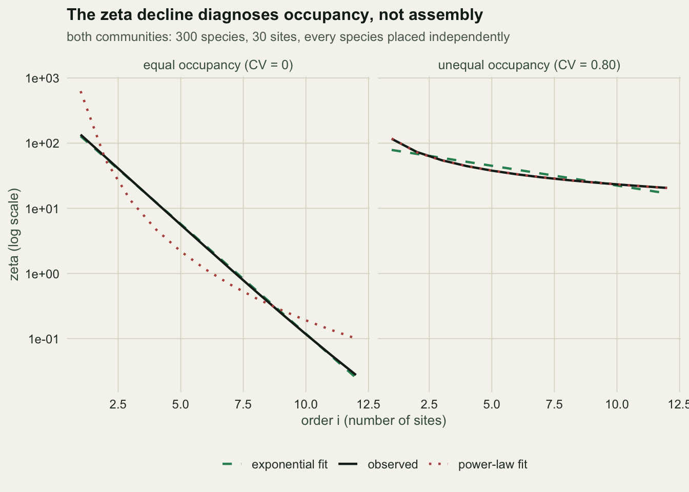
This is not a discovery, and it is not a flaw in the original paper. Hui and McGeoch (2014) say it in the body of their own text: null models in which species differ in their probability of occupying a site commonly produce the power-law form. The claim that survived into the citing literature is the abstract’s shorter version, and the caveat got left behind.
How much inequality is enough
The useful question is quantitative. How uneven do occupancy probabilities have to be before the power law takes over? Sweep the coefficient of variation and watch:
set.seed(3053)
dAIC_of <- function(z) {
  keep <- z > 0.5; ii <- which(keep); zz <- z[keep]
  if (length(zz) < 4) return(NA_real_)
  AIC(lm(log(zz) ~ ii)) - AIC(lm(log(zz) ~ log(ii)))
}

pars <- list(c(400, 600), c(40, 60), c(10, 15), c(4, 6), c(1.5, 2.25), c(0.8, 1.2), c(0.35, 0.55))
sweep_res <- do.call(rbind, lapply(pars, function(ab) {
  r <- replicate(12, {
    p <- rbeta(S, ab[1], ab[2])
    Xi <- matrix(rbinom(n_sites * S, 1, rep(p, each = n_sites)), n_sites, S)
    c(sd(p) / mean(p), dAIC_of(sapply(1:12, function(i) zeta(Xi, i))))
  })
  data.frame(cv = mean(r[1, ]), dAIC = mean(r[2, ], na.rm = TRUE), se = sd(r[2, ], na.rm = TRUE) / sqrt(12))
}))
sweep_res$verdict <- ifelse(sweep_res$dAIC > 2, "power law",
                     ifelse(sweep_res$dAIC < -2, "exponential", "tie"))
knitr::kable(sweep_res, digits = c(3, 1, 1, 0),
             col.names = c("CV of occupancy probability", "mean delta AIC (positive favours power law)",
"standard error", "verdict"))| CV of occupancy probability | mean delta AIC (positive favours power law) | standard error | verdict |
|---|---|---|---|
| 0.038 | -56.3 | 2.5 | exponential |
| 0.124 | -42.9 | 3.1 | exponential |
| 0.235 | -27.7 | 1.3 | exponential |
| 0.368 | -14.6 | 2.5 | exponential |
| 0.559 | 14.0 | 3.2 | power law |
| 0.699 | 31.0 | 3.2 | power law |
| 0.932 | 70.0 | 7.0 | power law |
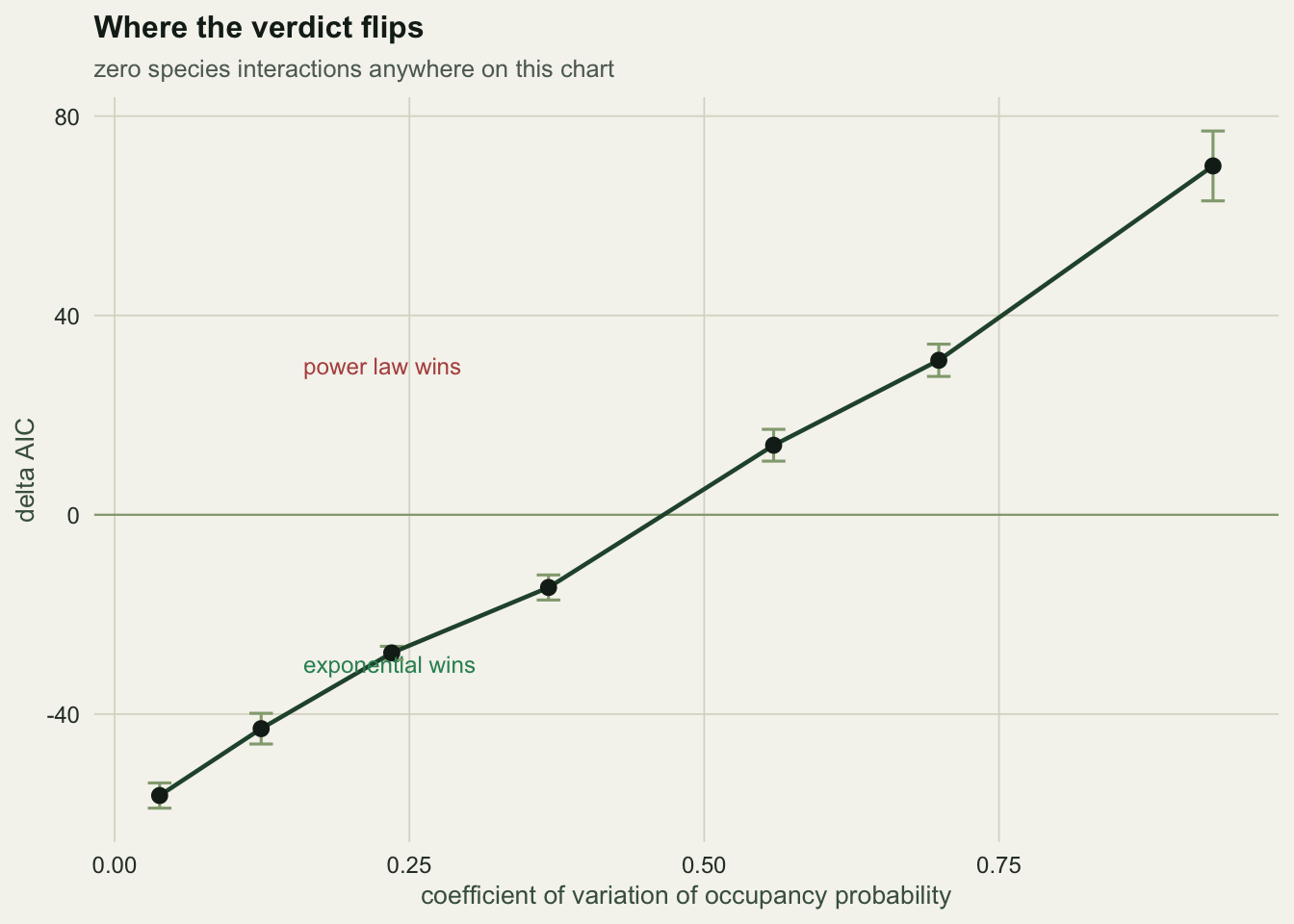
The crossover sits near a CV of 0.5. Real occupancy frequency distributions are routinely more uneven than that: most communities have a few species nearly everywhere and a long tail of species almost nowhere. In this simulation that much unevenness is enough for the exponential form to lose before any biology is involved, so in data with a similarly uneven occupancy distribution the power law’s win carries little information about assembly. Where exactly the crossover falls depends on the number of sites and the range of orders fitted.
McGlinn and Hurlbert (2012) made the same point from the other direction, showing that the scale dependence of species turnover tracks the variance of the occupancy frequency distribution. The decline form is a readout of that variance. It is a perfectly good readout. It is just not a readout of niches.
The retention ratio, which is more honest
If the decline form is over-interpreted, the ratio between consecutive orders is under-used. zeta_(i+1) / zeta_i is the probability that a species already shared by i sites is also in the next one:
ret <- function(z) z[-1] / z[-length(z)]
r_eq  <- ret(sapply(1:8, function(i) zeta(X_eq, i)))
r_het <- ret(sapply(1:8, function(i) zeta(X_het, i)))

knitr::kable(data.frame(step = paste0("zeta_", 2:8, " / zeta_", 1:7),
                        equal_occupancy = r_eq, unequal_occupancy = r_het),
digits = 3, col.names = c("step", "equal occupancy", "unequal occupancy"))| step | equal occupancy | unequal occupancy |
|---|---|---|
| zeta_2 / zeta_1 | 0.451 | 0.629 |
| zeta_3 / zeta_2 | 0.451 | 0.746 |
| zeta_4 / zeta_3 | 0.451 | 0.812 |
| zeta_5 / zeta_4 | 0.452 | 0.852 |
| zeta_6 / zeta_5 | 0.453 | 0.879 |
| zeta_7 / zeta_6 | 0.456 | 0.897 |
| zeta_8 / zeta_7 | 0.460 | 0.911 |
Under equal occupancy the retention ratio is flat, and it sits at 0.45, which recovers the p = 0.45 that generated the data. Under unequal occupancy it climbs, from 0.63 to 0.91, because each step drops the rarer species and leaves a progressively more common subset behind. That rise is the occupancy variance, expressed in a quantity with a meaning you can say out loud, rather than in a choice between two curve shapes.
Honest limits
Incidence only. Zeta counts species, not individuals. A site where a species is represented by one straggler counts identically to a site where it dominates. If your ecological question is about abundance structure, zeta cannot see it, and the multiplicative Hill beta at q = 2 can: multiplicative beta diversity.
The orders are not independent. zeta_5 is a deterministic function of the same occupancy vector that produced zeta_2. Fitting a curve across the orders and reading off standard errors or AIC differences treats them as independent observations; they are not, so the intervals will be too narrow and the AIC differences above overstate the strength of the evidence, though not the direction of the bend.
High orders need many sites. zeta_i for i near n averages over few subsets and swings wildly. The published advice is to read the decline over the low orders where you have data, and Hui and McGeoch (2014) fit theirs over a truncated range for exactly this reason.
Sampling. Zeta inherits every problem that incidence data has. A species missed at a site drops its occupancy, which drops every zeta above order 1 and inflates apparent turnover. See checking a beta diversity analysis.
Where to go next
Zeta answers the multi-site question that pairwise dissimilarity structurally cannot. Use it for that, report the retention ratios alongside the decline, and if you fit exponential against power law, report the occupancy distribution’s CV in the same table so a reader can see what is doing the work.
If you want a per-site number instead of a per-order one, the variance framing gives you that: beta diversity as variance.
References
Hui & McGeoch 2014 The American Naturalist 184(5):684-694 (10.1086/678125)
McGeoch, Latombe, Andrew, Nakagawa, Nipperess, Roige, Marzinelli, Campbell, Verges, Thomas, Steinberg, Selwood, Henriksen & Hui 2019 Ecology 100(11):e02832 (10.1002/ecy.2832)
McGlinn & Hurlbert 2012 Ecology 93(2):294-302 (10.1890/11-0229.1)